4.2: Statements of the Second Law

\( \newcommand{\tx}[1]{\text{#1}}      % text in math mode\)
 \( \newcommand{\subs}[1]{_{\text{#1}}} % subscript text\)
 \( \newcommand{\sups}[1]{^{\text{#1}}} % superscript text\)
 \( \newcommand{\st}{^\circ}            % standard state symbol\)
 \( \newcommand{\id}{^{\text{id}}}      % ideal\)
 \( \newcommand{\rf}{^{\text{ref}}}     % reference state\)
 \( \newcommand{\units}[1]{\mbox{$\thinspace$#1}}\)
 \( \newcommand{\K}{\units{K}}  % kelvins\)
 \( \newcommand{\degC}{^\circ\text{C}} % degrees Celsius\)
 \( \newcommand{\br}{\units{bar}}  % bar (\bar is already defined)\)
 \( \newcommand{\Pa}{\units{Pa}}\)
 \( \newcommand{\mol}{\units{mol}}  % mole\)
 \( \newcommand{\V}{\units{V}}  % volts\)
 \( \newcommand{\timesten}[1]{\mbox{$\,\times\,10^{#1}$}}\)
 \( \newcommand{\per}{^{-1}}  % minus one power\)
 \( \newcommand{\m}{_{\text{m}}}  % subscript m for molar quantity\)
 \( \newcommand{\CVm}{C_{V,\text{m}}} % molar heat capacity at const.V\)
 \( \newcommand{\Cpm}{C_{p,\text{m}}} % molar heat capacity at const.p\)
 \( \newcommand{\kT}{\kappa_T} % isothermal compressibility\)
 \( \newcommand{\A}{_{\text{A}}}  % subscript A for solvent or state A\)
 \( \newcommand{\B}{_{\text{B}}}  % subscript B for solute or state B\)
 \( \newcommand{\bd}{_{\text{b}}}  % subscript b for boundary or boiling point\)
 \( \newcommand{\C}{_{\text{C}}}  % subscript C\)
 \( \newcommand{\f}{_{\text{f}}}  % subscript f for freezing point\)
 \( \newcommand{\mA}{_{\text{m},\text{A}}} % subscript m,A (m=molar)\)
 \( \newcommand{\mB}{_{\text{m},\text{B}}} % subscript m,B (m=molar)\)
 \( \newcommand{\mi}{_{\text{m},i}}        % subscript m,i (m=molar)\)
 \( \newcommand{\fA}{_{\text{f},\text{A}}} % subscript f,A (for fr. pt.)\)
 \( \newcommand{\fB}{_{\text{f},\text{B}}} % subscript f,B (for fr. pt.)\)
 \( \newcommand{\xbB}{_{x,\text{B}}}       % x basis, B\)
 \( \newcommand{\xbC}{_{x,\text{C}}}       % x basis, C\)
 \( \newcommand{\cbB}{_{c,\text{B}}}       % c basis, B\)
 \( \newcommand{\mbB}{_{m,\text{B}}}       % m basis, B\)
 \( \newcommand{\kHi}{k_{\text{H},i}}      % Henry's law constant, x basis, i\)
 \( \newcommand{\kHB}{k_{\text{H,B}}}      % Henry's law constant, x basis, B\)
 \( \newcommand{\arrow}{\,\rightarrow\,} % right arrow with extra spaces\)
 \( \newcommand{\arrows}{\,\rightleftharpoons\,} % double arrows with extra spaces\)
 \( \newcommand{\ra}{\rightarrow} % right arrow (can be used in text mode)\)
 \( \newcommand{\eq}{\subs{eq}} % equilibrium state\)
 \( \newcommand{\onehalf}{\textstyle\frac{1}{2}\D} % small 1/2 for display equation\)
 \( \newcommand{\sys}{\subs{sys}} % system property\)
 \( \newcommand{\sur}{\sups{sur}} % surroundings\)
 \( \renewcommand{\in}{\sups{int}} % internal\)
 \( \newcommand{\lab}{\subs{lab}} % lab frame\)
 \( \newcommand{\cm}{\subs{cm}} % center of mass\)
 \( \newcommand{\rev}{\subs{rev}} % reversible\)
 \( \newcommand{\irr}{\subs{irr}} % irreversible\)
 \( \newcommand{\fric}{\subs{fric}} % friction\)
 \( \newcommand{\diss}{\subs{diss}} % dissipation\)
 \( \newcommand{\el}{\subs{el}} % electrical\)
 \( \newcommand{\cell}{\subs{cell}} % cell\)
 \( \newcommand{\As}{A\subs{s}} % surface area\)
 \( \newcommand{\E}{^\mathsf{E}} % excess quantity (superscript)\)
 \( \newcommand{\allni}{\{n_i \}} % set of all n_i\)
 \( \newcommand{\sol}{\hspace{-.1em}\tx{(sol)}}\)
 \( \newcommand{\solmB}{\tx{(sol,$\,$$m\B$)}}\)
 \( \newcommand{\dil}{\tx{(dil)}}\)
 \( \newcommand{\sln}{\tx{(sln)}}\)
 \( \newcommand{\mix}{\tx{(mix)}}\)
 \( \newcommand{\rxn}{\tx{(rxn)}}\)
 \( \newcommand{\expt}{\tx{(expt)}}\)
 \( \newcommand{\solid}{\tx{(s)}}\)
 \( \newcommand{\liquid}{\tx{(l)}}\)
 \( \newcommand{\gas}{\tx{(g)}}\)
 \( \newcommand{\pha}{\alpha}        % phase alpha\)
 \( \newcommand{\phb}{\beta}         % phase beta\)
 \( \newcommand{\phg}{\gamma}        % phase gamma\)
 \( \newcommand{\aph}{^{\alpha}}     % alpha phase superscript\)
 \( \newcommand{\bph}{^{\beta}}      % beta phase superscript\)
 \( \newcommand{\gph}{^{\gamma}}     % gamma phase superscript\)
 \( \newcommand{\aphp}{^{\alpha'}}   % alpha prime phase superscript\)
 \( \newcommand{\bphp}{^{\beta'}}    % beta prime phase superscript\)
 \( \newcommand{\gphp}{^{\gamma'}}   % gamma prime phase superscript\)
 \( \newcommand{\apht}{\small\aph} % alpha phase tiny superscript\)
 \( \newcommand{\bpht}{\small\bph} % beta phase tiny superscript\)
 \( \newcommand{\gpht}{\small\gph} % gamma phase tiny superscript\)

\( \newcommand{\upOmega}{\Omega}\)

 \( \newcommand{\dif}{\mathop{}\!\mathrm{d}}   % roman d in math mode, preceded by space\)
 \( \newcommand{\Dif}{\mathop{}\!\mathrm{D}}   % roman D in math mode, preceded by space\)
 \( \newcommand{\df}{\dif\hspace{0.05em} f} % df\)

 \(\newcommand{\dBar}{\mathop{}\!\mathrm{d}\hspace-.3em\raise1.05ex{\Rule{.8ex}{.125ex}{0ex}}} % inexact differential \)
 \( \newcommand{\dq}{\dBar q} % heat differential\)
 \( \newcommand{\dw}{\dBar w} % work differential\)
 \( \newcommand{\dQ}{\dBar Q} % infinitesimal charge\)
 \( \newcommand{\dx}{\dif\hspace{0.05em} x} % dx\)
 \( \newcommand{\dt}{\dif\hspace{0.05em} t} % dt\)
 \( \newcommand{\difp}{\dif\hspace{0.05em} p} % dp\)
 \( \newcommand{\Del}{\Delta}\)
 \( \newcommand{\Delsub}[1]{\Delta_{\text{#1}}}\)
 \( \newcommand{\pd}[3]{(\partial #1 / \partial #2 )_{#3}} % \pd{}{}{} - partial derivative, one line\)
 \( \newcommand{\Pd}[3]{\left( \dfrac {\partial #1} {\partial #2}\right)_{#3}} % Pd{}{}{} - Partial derivative, built-up\)
 \( \newcommand{\bpd}[3]{[ \partial #1 / \partial #2 ]_{#3}}\)
 \( \newcommand{\bPd}[3]{\left[ \dfrac {\partial #1} {\partial #2}\right]_{#3}}\)
 \( \newcommand{\dotprod}{\small\bullet}\)
 \( \newcommand{\fug}{f} % fugacity\)
 \( \newcommand{\g}{\gamma} % solute activity coefficient, or gamma in general\)
 \( \newcommand{\G}{\varGamma} % activity coefficient of a reference state (pressure factor)\)
 \( \newcommand{\ecp}{\widetilde{\mu}} % electrochemical or total potential\)
 \( \newcommand{\Eeq}{E\subs{cell, eq}} % equilibrium cell potential\)
 \( \newcommand{\Ej}{E\subs{j}} % liquid junction potential\)
 \( \newcommand{\mue}{\mu\subs{e}} % electron chemical potential\)
\( \newcommand{\defn}{\,\stackrel{\mathrm{def}}{=}\,} % "equal by definition" symbol\)

 \( \newcommand{\D}{\displaystyle} % for a line in built-up\)
 \( \newcommand{\s}{\smash[b]} % use in equations with conditions of validity\)
 \( \newcommand{\cond}[1]{\\[-2.5pt]{}\tag*{#1}}\)
 \( \newcommand{\nextcond}[1]{\\[-5pt]{}\tag*{#1}}\)
 \( \newcommand{\R}{8.3145\units{J$\,$K$\per\,$mol$\per$}}     % gas constant value\)
 \( \newcommand{\Rsix}{8.31447\units{J$\,$K$\per\,$mol$\per$}} % gas constant value - 6 sig figs\)

\( \newcommand{\jn}{\hspace3pt\lower.3ex{\Rule{.6pt}{2ex}{0ex}}\hspace3pt} \)
\( \newcommand{\ljn}{\hspace3pt\lower.3ex{\Rule{.6pt}{.5ex}{0ex}}\hspace-.6pt\raise.45ex{\Rule{.6pt}{.5ex}{0ex}}\hspace-.6pt\raise1.2ex{\Rule{.6pt}{.5ex}{0ex}} \hspace3pt} \)
\( \newcommand{\lljn}{\hspace3pt\lower.3ex{\Rule{.6pt}{.5ex}{0ex}}\hspace-.6pt\raise.45ex{\Rule{.6pt}{.5ex}{0ex}}\hspace-.6pt\raise1.2ex{\Rule{.6pt}{.5ex}{0ex}}\hspace1.4pt\lower.3ex{\Rule{.6pt}{.5ex}{0ex}}\hspace-.6pt\raise.45ex{\Rule{.6pt}{.5ex}{0ex}}\hspace-.6pt\raise1.2ex{\Rule{.6pt}{.5ex}{0ex}}\hspace3pt} \) 

A description of the mathematical statement of the second law is given in the box below.

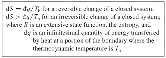
The box includes three distinct parts. First, there is the assertion that a property called entropy, \(S\), is an extensive state function.

Second, there is an equation for calculating the entropy change of a closed system during a reversible change of state: \(\dif S\) is equal to \(\dq/T\bd\). During a reversible process, the temperature usually has the same value \(T\) throughout the system, in which case we can simply write \(\dif S = \dq/T\). The equation \(\dif S = \dq/T\bd\) allows for the possibility that in an equilibrium state the system has phases of different temperatures separated by internal adiabatic partitions.

Third, there is a criterion for spontaneity: \(\dif S\) is greater than \(\dq/T\bd\) during an irreversible change of state. The temperature \(T\bd\) is a thermodynamic temperature, which will be defined in Sec. 4.3.4.

Each of the three parts is an essential component of the second law, but is somewhat abstract. What fundamental principle, based on experimental observation, may we take as the starting point to obtain them? Two principles are available, one associated with Clausius and the other with Kelvin and Planck. Both principles are equivalent statements of the second law. Each asserts that a certain kind of process is impossible, in agreement with common experience.

Next consider the impossible process shown in Fig. 4.2(a). A Joule paddle wheel rotates in a container of water as a weight rises. As the weight gains potential energy, the water loses thermal energy and its temperature decreases. Energy is conserved, so there is no violation of the first law. This process is just the reverse of the Joule paddle-wheel experiment (Sec. 3.7.2) and its impossibility has already been discussed.

We might again attempt to use some sort of device operating in a cycle to accomplish the same overall process, as in Fig. 4.2(b). A closed system that operates in a cycle and does net work on the surroundings is called a heat engine. The heat engine shown in Fig. 4.2(b) is a special one. During one cycle, a quantity of energy is transferred by heat from a heat reservoir to the engine, and the engine performs an equal quantity of work on a weight, causing it to rise. At the end of the cycle, the engine has returned to its initial state. This would be a very desirable engine, because it could convert thermal energy into an equal quantity of useful mechanical work with no other effect on the surroundings. (This hypothetical process is called “perpetual motion of the second kind.”) The engine could power a ship; it would use the ocean as a heat reservoir and require no fuel. Unfortunately, it is impossible to construct such a heat engine!

The principle was expressed by William Thomson (Lord Kelvin) in 1852 as follows: “It is impossible by means of inanimate material agency to derive mechanical effect from any portion of matter by cooling it below the temperature of the coldest of the surrounding objects.” Max Planck in 1922 gave this statement: “It is impossible to construct an engine which will work in a complete cycle, and produce no effect except the raising of a weight and the cooling of a heat-reservoir.” For the purposes of this chapter, the principle can be reworded as follows.

• Both the Clausius statement and the Kelvin–Planck statement assert that certain processes, although they do not violate the first law, are nevertheless impossible.

  These processes would not be impossible if we could control the trajectories of large numbers of individual particles. Newton’s laws of motion are invariant to time reversal. Suppose we could measure the position and velocity of each molecule of a macroscopic system in the final state of an irreversible process. Then, if we could somehow arrange at one instant to place each molecule in the same position with its velocity reversed, and if the molecules behaved classically, they would retrace their trajectories in reverse and we would observe the reverse “impossible” process.

  Carnot engines and Carnot cycles are admittedly outside the normal experience of chemists, and using them to derive the mathematical statement of the second law may seem arcane. G. N. Lewis and M. Randall, in their classic 1923 book Thermodynamics and the Free Energy of Chemical Substances, complained of the presentation of “cyclical processes limping about eccentric and not quite completed cycles.” There seems, however, to be no way to carry out a rigorous general derivation without invoking thermodynamic cycles. You may avoid the details by skipping Secs. 4.3–4.5. (Incidently, the cycles described in these sections are complete!)