
16.3: Classical Treatment of Nuclear Motion
- Page ID
- 60584

\( \newcommand{\vecs}[1]{\overset { \scriptstyle \rightharpoonup} {\mathbf{#1}} } \)
\( \newcommand{\vecd}[1]{\overset{-\!-\!\rightharpoonup}{\vphantom{a}\smash {#1}}} \)
\( \newcommand{\dsum}{\displaystyle\sum\limits} \)
\( \newcommand{\dint}{\displaystyle\int\limits} \)
\( \newcommand{\dlim}{\displaystyle\lim\limits} \)
\( \newcommand{\id}{\mathrm{id}}\) \( \newcommand{\Span}{\mathrm{span}}\)
( \newcommand{\kernel}{\mathrm{null}\,}\) \( \newcommand{\range}{\mathrm{range}\,}\)
\( \newcommand{\RealPart}{\mathrm{Re}}\) \( \newcommand{\ImaginaryPart}{\mathrm{Im}}\)
\( \newcommand{\Argument}{\mathrm{Arg}}\) \( \newcommand{\norm}[1]{\| #1 \|}\)
\( \newcommand{\inner}[2]{\langle #1, #2 \rangle}\)
\( \newcommand{\Span}{\mathrm{span}}\)
\( \newcommand{\id}{\mathrm{id}}\)
\( \newcommand{\Span}{\mathrm{span}}\)
\( \newcommand{\kernel}{\mathrm{null}\,}\)
\( \newcommand{\range}{\mathrm{range}\,}\)
\( \newcommand{\RealPart}{\mathrm{Re}}\)
\( \newcommand{\ImaginaryPart}{\mathrm{Im}}\)
\( \newcommand{\Argument}{\mathrm{Arg}}\)
\( \newcommand{\norm}[1]{\| #1 \|}\)
\( \newcommand{\inner}[2]{\langle #1, #2 \rangle}\)
\( \newcommand{\Span}{\mathrm{span}}\) \( \newcommand{\AA}{\unicode[.8,0]{x212B}}\)
\( \newcommand{\vectorA}[1]{\vec{#1}} % arrow\)
\( \newcommand{\vectorAt}[1]{\vec{\text{#1}}} % arrow\)
\( \newcommand{\vectorB}[1]{\overset { \scriptstyle \rightharpoonup} {\mathbf{#1}} } \)
\( \newcommand{\vectorC}[1]{\textbf{#1}} \)
\( \newcommand{\vectorD}[1]{\overrightarrow{#1}} \)
\( \newcommand{\vectorDt}[1]{\overrightarrow{\text{#1}}} \)
\( \newcommand{\vectE}[1]{\overset{-\!-\!\rightharpoonup}{\vphantom{a}\smash{\mathbf {#1}}}} \)
\( \newcommand{\vecs}[1]{\overset { \scriptstyle \rightharpoonup} {\mathbf{#1}} } \)
\(\newcommand{\longvect}{\overrightarrow}\)
\( \newcommand{\vecd}[1]{\overset{-\!-\!\rightharpoonup}{\vphantom{a}\smash {#1}}} \)
\(\newcommand{\avec}{\mathbf a}\) \(\newcommand{\bvec}{\mathbf b}\) \(\newcommand{\cvec}{\mathbf c}\) \(\newcommand{\dvec}{\mathbf d}\) \(\newcommand{\dtil}{\widetilde{\mathbf d}}\) \(\newcommand{\evec}{\mathbf e}\) \(\newcommand{\fvec}{\mathbf f}\) \(\newcommand{\nvec}{\mathbf n}\) \(\newcommand{\pvec}{\mathbf p}\) \(\newcommand{\qvec}{\mathbf q}\) \(\newcommand{\svec}{\mathbf s}\) \(\newcommand{\tvec}{\mathbf t}\) \(\newcommand{\uvec}{\mathbf u}\) \(\newcommand{\vvec}{\mathbf v}\) \(\newcommand{\wvec}{\mathbf w}\) \(\newcommand{\xvec}{\mathbf x}\) \(\newcommand{\yvec}{\mathbf y}\) \(\newcommand{\zvec}{\mathbf z}\) \(\newcommand{\rvec}{\mathbf r}\) \(\newcommand{\mvec}{\mathbf m}\) \(\newcommand{\zerovec}{\mathbf 0}\) \(\newcommand{\onevec}{\mathbf 1}\) \(\newcommand{\real}{\mathbb R}\) \(\newcommand{\twovec}[2]{\left[\begin{array}{r}#1 \\ #2 \end{array}\right]}\) \(\newcommand{\ctwovec}[2]{\left[\begin{array}{c}#1 \\ #2 \end{array}\right]}\) \(\newcommand{\threevec}[3]{\left[\begin{array}{r}#1 \\ #2 \\ #3 \end{array}\right]}\) \(\newcommand{\cthreevec}[3]{\left[\begin{array}{c}#1 \\ #2 \\ #3 \end{array}\right]}\) \(\newcommand{\fourvec}[4]{\left[\begin{array}{r}#1 \\ #2 \\ #3 \\ #4 \end{array}\right]}\) \(\newcommand{\cfourvec}[4]{\left[\begin{array}{c}#1 \\ #2 \\ #3 \\ #4 \end{array}\right]}\) \(\newcommand{\fivevec}[5]{\left[\begin{array}{r}#1 \\ #2 \\ #3 \\ #4 \\ #5 \\ \end{array}\right]}\) \(\newcommand{\cfivevec}[5]{\left[\begin{array}{c}#1 \\ #2 \\ #3 \\ #4 \\ #5 \\ \end{array}\right]}\) \(\newcommand{\mattwo}[4]{\left[\begin{array}{rr}#1 \amp #2 \\ #3 \amp #4 \\ \end{array}\right]}\) \(\newcommand{\laspan}[1]{\text{Span}\{#1\}}\) \(\newcommand{\bcal}{\cal B}\) \(\newcommand{\ccal}{\cal C}\) \(\newcommand{\scal}{\cal S}\) \(\newcommand{\wcal}{\cal W}\) \(\newcommand{\ecal}{\cal E}\) \(\newcommand{\coords}[2]{\left\{#1\right\}_{#2}}\) \(\newcommand{\gray}[1]{\color{gray}{#1}}\) \(\newcommand{\lgray}[1]{\color{lightgray}{#1}}\) \(\newcommand{\rank}{\operatorname{rank}}\) \(\newcommand{\row}{\text{Row}}\) \(\newcommand{\col}{\text{Col}}\) \(\renewcommand{\row}{\text{Row}}\) \(\newcommand{\nul}{\text{Nul}}\) \(\newcommand{\var}{\text{Var}}\) \(\newcommand{\corr}{\text{corr}}\) \(\newcommand{\len}[1]{\left|#1\right|}\) \(\newcommand{\bbar}{\overline{\bvec}}\) \(\newcommand{\bhat}{\widehat{\bvec}}\) \(\newcommand{\bperp}{\bvec^\perp}\) \(\newcommand{\xhat}{\widehat{\xvec}}\) \(\newcommand{\vhat}{\widehat{\vvec}}\) \(\newcommand{\uhat}{\widehat{\uvec}}\) \(\newcommand{\what}{\widehat{\wvec}}\) \(\newcommand{\Sighat}{\widehat{\Sigma}}\) \(\newcommand{\lt}{<}\) \(\newcommand{\gt}{>}\) \(\newcommand{\amp}{&}\) \(\definecolor{fillinmathshade}{gray}{0.9}\)For all but very elementary chemical reactions (e.g., D + HH \(\rightarrow\) HD + H or F + HH \(\rightarrow\) FH + H) or scattering processes (e.g., CO (v,J) + He \(\rightarrow\) CO (v',J') + He), the above fully quantal coupled equations simply can not be solved even when modern supercomputers are employed.Fortunately, the Schrödinger equation can be replaced by a simple classical mechanics treatment of nuclear motions under certain circumstances.
For motion of a particle of mass \(\mu\) along a direction R, the primary condition under which a classical treatment of nuclear motion is valid
\[ \dfrac{\lambda}{4\pi}\dfrac{1}{\text{p}}\bigg|\dfrac{\text{dp}}{\text{dR}}\bigg| \ll 1 \nonumber \]
relates to the fractional change in the local momentum defined as:
\[ \text{p} = \sqrt{2\mu (\text{E - E}_j\text{(R)})} \nonumber \]
along R within the 3N - 5 or 3N - 6 dimensional internal coordinate space of the molecule, as well as to the local de Broglie wavelength
\[ \lambda = \dfrac{2\pi\hbar}{|\text{p}|}. \nonumber \]
The inverse of the quantity \( \dfrac{1}{\text{p}}\bigg| \dfrac{\text{dp}}{\text{dR}} \bigg| \) can be thought of as the length over which the momentum changes by 100%. The above condition then states that the local de Broglie wavelength must be short with respect to the distance over which the potential changes appreciably. Clearly, whenever one is dealing with heavy nuclei that are moving fast (so |p| is large), one should anticipate that the local de Broglie wavelength of those particles may be short enough to meet the above criteria for classical treatment.
It has been determined that for potentials characteristic of typical chemical bonding (whose depths and dynamic range of interatomic distances are well known), and for all but low-energy motions (e.g., zero-point vibrations) of light particles such as Hydrogen and Deuterium nuclei or electrons, the local de Broglie wavelengths are often short enough for the above condition to be met (because of the large masses \(\mu\) of non-Hydrogenic species) except when their velocities approach zero (e.g., near classical turning points). It is therefore common to treat the nuclear-motion dynamics of molecules that do not contain H or D atoms in a purely classical manner, and to apply so-called semi-classical corrections near classical turning points. The motions of H and D atomic centers usually require quantal treatment except when their kinetic energies are quite high.
Classical Trajectories
To apply classical mechanics to the treatment of nuclear-motion dynamics, one solves Newtonian equations
\[ \text{m}_{\text{k}}\dfrac{\text{d}^2\text{X}_{\text{k}}}{\text{dt}^2} = - \dfrac{\text{dE}_{\text{j}}}{\text{dX}_{\text{k}}} \nonumber \]
where \(\text{X}_{\text{k}}\) denotes one of the 3N cartesian coordinates of the atomic centers in the molecule, m\(_{\text{k}}\) is the mass of the atom associated with this coordinate, and \( \frac{\text{dE}_{\text{j}}}{\text{dX}_{\text{k}}} \) is the derivative of the potential, which is the electronic energy \(\text{E}_{\text{j}}\)(R), along the \(\text{k}^{\text{th}}\) coordinate's direction. Starting with coordinates {\(\text{X}_{\text{k}}\)(0)} and corresponding momenta {\(\text{P}_{\text{k}}\)(0)} at some initial time t = 0, and given the ability to compute the force - \( \frac{\text{dE}_{\text{j}}}{\text{dX}_{\text{k}}} \) at any location of the nuclei, the Newton equations can be solved (usually on a computer) using finite-difference methods:
\[ \text{X}_{\text{k}}(t+\delta t) = \text{X}_{text{k}}(t) + \text{P}_{\text{k}}(t) \dfrac{\delta t}{\text{m}_{\text{k}}} \nonumber \]
\[ \text{P}_{\text{k}}(t+\delta t) = \text{P}_{\text{k}}(t) - \dfrac{\text{dE}_j}{\text{dX}_k}(t) \delta t. \nonumber \]
In so doing, one generates a sequence of coordinates {\(\text{X}_k(\text{t}_n)\)} and momenta {\(\text{P}_k(\text{t}_n)\)}, one for each "time step" tn. The histories of these coordinates and momenta as functions of time are called "classical trajectories". Following them from early times, characteristic of the molecule(s) at "reactant" geometries, through to late times, perhaps characteristic of "product" geometries, allows one to monitor and predict the fate of the time evolution of the nuclear dynamics. Even for large molecules with many atomic centers, propagation of such classical trajectories is feasible on modern computers if the forces - \( \frac{\text{dE}_j}{\text{dX}_k} \) can be computed in a manner that does not consume inordinate amounts of computer time.
In Section 6, methods by which such force calculations are performed using firstprinciples quantum mechanical methods (i.e., so-called ab initio methods) are discussed. Suffice it to say that these calculations are often the rate limiting step in carrying out classical trajectory simulations of molecular dynamics. The large effort involved in the ab initio determination of electronic energies and their gradients - \(\frac{\text{dE}}{\text{dX}_k}\) motivate one to consider using empirical "force field" functions V\(_j\) (R) in place of the ab initio electronic energy E\(_j\) (R). Such model potentials V\)_j\) (R), are usually constructed in terms of easy to compute and to differentiate functions of the interatomic distances and valence angles that appear in the molecule. The parameters that appear in the attractive and repulsive parts of these potentials are usually chosen so the potential is consistent with certain experimental data (e.g., bond dissociation energies, bond lengths, vibrational energies, torsion energy barriers).
For a large polyatomic molecule, the potential function V usually contains several distinct contributions:
\[ V = V_{\text{bond}^+} V_{\text{bend}^+} V_{\text{vanderWaals}^+}V_{\text{torsion}^+}V_{\text{electrostatic}}. \nonumber \]
Here \(\text{V}_{\text{bond}}\) gives the dependence of V on stretching displacements of the bonds (i.e., interatomic distances between pairs of bonded atoms) and is usually modeled as a harmonic or Morse function for each bond in the molecule:
\[ \text{V}_{\text{bond}} = \sum\limits_J \dfrac{1}{2}k_j (R_j - R_{\text{eq,J}})^2 \nonumber \]
or
\[ \text{V}_{\text{bond}} = \sum\limits_J \text{D}_{\text{e,J}} \left( 1-e^{-a_J(\text{R}_J - \text{R}_{\text{eq,J }) }} \right)^2 \nonumber \]
where the index J labels the bonds and the \(k_J \text{ , } a_J \text{ and } R_{eq,J}\) are the force constant and equilibrium bond length parameters for the \(J^{th}\) bond.
\(\text{V}_{\text{bend}}\) describes the bending potentials for each triplet of atoms (ABC) that are bonded in a A-B-C manner; it is usually modeled in terms of a harmonic potential for each such bend:
\[ \text{V}_{\text{bend}} = \sum\limits_J \dfrac{1}{2}k^{\theta}_{J}\left( \theta_J - \theta_{\text{eq,J}} \right)^2. \nonumber \]
The \(\theta_{\text{eq,J}} \text{ and } k^{\theta}_J\) are the equilibrium angles and force constants for the J\(^{th}\) angle.
\(\text{V}_{\text{vanderWaals}}\) represents the van der Waals interactions between all pairs of atoms that are not bonded to one another. It is usually written as a sum over all pairs of such atoms (labeled J and K) of a Lennard-Jones 6-12 potential:
\[ \text{V}_{\text{vanderWaals}} = \sum\limits_{J<k} \left[ a_{J,K}(R_{J,K})^{-12} - b_{J,K}(R_{J,K})^{-6} \right] \nonumber \]
where \(a_{J,K} \text{ and } b_{J,K}\) are parameters relating to the repulsive and dispersion attraction forces, respectively for the \(\text{J}^{\text{th}} \text{ and } \text{K}^{\text{th}}\) atoms.
\(\text{V}_{\text{torsion}}\) contributions describe the dependence of V on angles of rotation about single bonds. For example, rotation of a CH\(_3\) group around the single bond connecting the carbon atom to another group may have an angle dependence of the form:
\[ \text{V}_{\text{torsion}} = V_0(1 - cos(3\theta)) \nonumber \]
where \(\theta\) is the torsion rotation angle, and \(V_0\) is the magnitude of the interaction between the C-H bonds and the group on the atom bonded to carbon.
\(\text{V}_{\text{electrostatic}}\) contains the interactions among polar bonds or other polar groups (including any charged groups). It is usually written as a sum over pairs of atomic centers (J and K) of Coulombic interactions between fractional charges {Q\(_J\)} (chosen to represent the bond polarity) on these atoms:
\[ \text{V}_{\text{electrostatic}} = \sum\limits_{J<K}\dfrac{\text{Q}_J\text{Q}_K}{\text{R}_{J,K}} \nonumber \]
Although the total potential V as written above contains many components, each is a relatively simple function of the Cartesian positions of the atomic centers. Therefore, it is relatively straightforward to evaluate V and its gradient along all 3N Cartesian directions in a computationally efficient manner. For this reason, the use of such empirical force fields in so-called molecular mechanics simulations of classical dynamics is widely used for treating large organic and biological molecules.
Initial Conditions
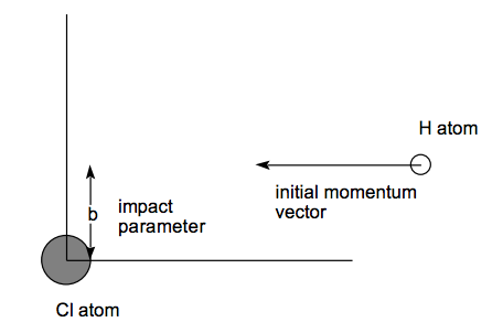
No single trajectory can be used to simulate chemical reaction or collisions that relate to realistic experiments. To generate classical trajectories that are characteristic of particular experiments, one must choose many initial conditions (coordinates and momenta) the collection of which is representative of the experiment. For example, to use an ensemble of trajectories to simulate a molecular beam collision between H and Cl atoms at a collision energy E, one must follow many classical trajectories that have a range of "impact parameters" (b) from zero up to some maximum value b\(_{max}\) beyond which the H ....Cl interaction potential vanishes. The figure shown below describes the impact parameter as the distance of closest approach that a trajectory would have if no attractive or repulsive forces were operative.
Moreover, if the energy resolution of the experiment makes it impossible to fix the collision energy closer than an amount \(\delta\)E, one must run collections of trajectories for values of E lying within this range.
If, in contrast, one wishes to simulate thermal reaction rates, one needs to follow trajectories with various E values and various impact parameters b from initiation at t = 0 to their conclusion (at which time the chemical outcome is interrogated). Each of these trajectories must have their outcome weighted by an amount proportional to a Boltzmann factor \( e^{\frac{-E}{RT}} \), where R is the ideal gas constant and T is the temperature because this factor specifies the probability that a collision occurs with kinetic energy E.
As the complexity of the molecule under study increases, the number of parameters needed to specify the initial conditions also grows. For example, classical trajectories that relate to \(\text{F + H}_2 \rightarrow \text{ HF + H }\) need to be specified by providing (i) an impact parameter for the F to the center of mass of \(\text{H}_2\), (ii) the relative translational energy of the F and \(\text{H}_2\), (iii) the radial momentum and coordinate of the \(\text{H}_2\) molecule's bond length, and (iv) the angular momentum of the \(\text{H}_2\) molecule as well as the angle of the H-H bond axis relative to the line connecting the F atom to the center of mass of the \(\text{H}_2\) molecule. Many such sets of initial conditions must be chosen and the resultant classical trajectories followed to generate an ensemble of trajectories pertinent to an experimental situation.
It should be clear that even the classical mechanical simulation of chemical experiments involves considerable effort because no single trajectory can represent the experimental situation. Many trajectories, each with different initial conditions selected so they represent, as an ensemble, the experimental conditions, must be followed and the outcome of all such trajectories must be averaged over the probability of realizing each specific initial condition.
Analyzing Final Conditions
Even after classical trajectories have been followed from t = 0 until the outcomes of the collisions are clear, one needs to properly relate the fate of each trajectory to the experimental situation. For the \(\text{F + H}_2 \rightarrow \text{ HF + H}\) example used above, one needs to examine each trajectory to determine, for example, (i) whether HF + H products are formed or non-reactive collision to produce F + \(\text{H}_2\) has occurred, (ii) the amount of rotational energy and angular momentum that is contained in the HF product molecule, (iii) the amount of relative translational energy that remains in the H + FH products, and (iv) the amount of vibrational energy that ends up in the HF product molecule.
Because classical rather than quantum mechanical equations are used to follow the time evolution of the molecular system, there is no guarantee that the amount of energy or angular momentum found in degrees of freedom for which these quantities should be quantized will be so. For example, \(\text{ F + H}_2 \rightarrow \text{ HF + H }\) trajectories may produce HF molecules with internal vibrational energy that is not a half integral multiple of the fundamental vibrational frequency w of the HF bond. Also, the rotational angular momentum of the HF molecule may not fit the formula \( J(J+1)\frac{h^2}{8\pi^2I} \), where I is HF's moment of inertia.
To connect such purely classical mechanical results more closely to the world of quantized energy levels, a method know as "binning" is often used. In this technique, one assigns the outcome of a classical trajectory to the particular quantum state (e.g., to a vibrational state v or a rotational state J of the HF molecule in the above example) whose quantum energy is closest to the classically determined energy. For the HF example at hand, the classical vibrational energy \(\text{E}_{\text{cl.vib}}\) is simply used to define, as the closest integer, a vibrational quantum number v according to:
\[ v = \dfrac{\text{E}_{\text{cl.vib}}}{\hbar\omega}-\dfrac{1}{2}. \nonumber \]
Likewise, a rotational quantum number J can be assigned as the closest integer to that determined by using the classical rotational energy \(\text{E}_{\text{cl.vib}}\) in the formula:
\[ J = \dfrac{1}{2}\left[ \sqrt{1+\dfrac{32\pi^2IE_{\text{cl,rot}}}{h^2}} -1 \right] \nonumber \]
which is the solution of the quadratic equation \( J(J+1)\frac{h^2}{8\pi^2I} = \text{E}_{\text{cl,rot}} \) By following many trajectories and assigning vibrational and rotational quantum numbers to the product molecules formed in each trajectory, one can generate histograms giving the frequency with which each product molecule quantum state is observed for the ensemble of trajectories used to simulate the experiment of interest. In this way, one can approximately extract product-channel quantum state distributions from classical trajectory simulations.