
12.8.1: Shear Viscosity
- Page ID
- 5283

\( \newcommand{\vecs}[1]{\overset { \scriptstyle \rightharpoonup} {\mathbf{#1}} } \)
\( \newcommand{\vecd}[1]{\overset{-\!-\!\rightharpoonup}{\vphantom{a}\smash {#1}}} \)
\( \newcommand{\id}{\mathrm{id}}\) \( \newcommand{\Span}{\mathrm{span}}\)
( \newcommand{\kernel}{\mathrm{null}\,}\) \( \newcommand{\range}{\mathrm{range}\,}\)
\( \newcommand{\RealPart}{\mathrm{Re}}\) \( \newcommand{\ImaginaryPart}{\mathrm{Im}}\)
\( \newcommand{\Argument}{\mathrm{Arg}}\) \( \newcommand{\norm}[1]{\| #1 \|}\)
\( \newcommand{\inner}[2]{\langle #1, #2 \rangle}\)
\( \newcommand{\Span}{\mathrm{span}}\)
\( \newcommand{\id}{\mathrm{id}}\)
\( \newcommand{\Span}{\mathrm{span}}\)
\( \newcommand{\kernel}{\mathrm{null}\,}\)
\( \newcommand{\range}{\mathrm{range}\,}\)
\( \newcommand{\RealPart}{\mathrm{Re}}\)
\( \newcommand{\ImaginaryPart}{\mathrm{Im}}\)
\( \newcommand{\Argument}{\mathrm{Arg}}\)
\( \newcommand{\norm}[1]{\| #1 \|}\)
\( \newcommand{\inner}[2]{\langle #1, #2 \rangle}\)
\( \newcommand{\Span}{\mathrm{span}}\) \( \newcommand{\AA}{\unicode[.8,0]{x212B}}\)
\( \newcommand{\vectorA}[1]{\vec{#1}} % arrow\)
\( \newcommand{\vectorAt}[1]{\vec{\text{#1}}} % arrow\)
\( \newcommand{\vectorB}[1]{\overset { \scriptstyle \rightharpoonup} {\mathbf{#1}} } \)
\( \newcommand{\vectorC}[1]{\textbf{#1}} \)
\( \newcommand{\vectorD}[1]{\overrightarrow{#1}} \)
\( \newcommand{\vectorDt}[1]{\overrightarrow{\text{#1}}} \)
\( \newcommand{\vectE}[1]{\overset{-\!-\!\rightharpoonup}{\vphantom{a}\smash{\mathbf {#1}}}} \)
\( \newcommand{\vecs}[1]{\overset { \scriptstyle \rightharpoonup} {\mathbf{#1}} } \)
\( \newcommand{\vecd}[1]{\overset{-\!-\!\rightharpoonup}{\vphantom{a}\smash {#1}}} \)
\(\newcommand{\avec}{\mathbf a}\) \(\newcommand{\bvec}{\mathbf b}\) \(\newcommand{\cvec}{\mathbf c}\) \(\newcommand{\dvec}{\mathbf d}\) \(\newcommand{\dtil}{\widetilde{\mathbf d}}\) \(\newcommand{\evec}{\mathbf e}\) \(\newcommand{\fvec}{\mathbf f}\) \(\newcommand{\nvec}{\mathbf n}\) \(\newcommand{\pvec}{\mathbf p}\) \(\newcommand{\qvec}{\mathbf q}\) \(\newcommand{\svec}{\mathbf s}\) \(\newcommand{\tvec}{\mathbf t}\) \(\newcommand{\uvec}{\mathbf u}\) \(\newcommand{\vvec}{\mathbf v}\) \(\newcommand{\wvec}{\mathbf w}\) \(\newcommand{\xvec}{\mathbf x}\) \(\newcommand{\yvec}{\mathbf y}\) \(\newcommand{\zvec}{\mathbf z}\) \(\newcommand{\rvec}{\mathbf r}\) \(\newcommand{\mvec}{\mathbf m}\) \(\newcommand{\zerovec}{\mathbf 0}\) \(\newcommand{\onevec}{\mathbf 1}\) \(\newcommand{\real}{\mathbb R}\) \(\newcommand{\twovec}[2]{\left[\begin{array}{r}#1 \\ #2 \end{array}\right]}\) \(\newcommand{\ctwovec}[2]{\left[\begin{array}{c}#1 \\ #2 \end{array}\right]}\) \(\newcommand{\threevec}[3]{\left[\begin{array}{r}#1 \\ #2 \\ #3 \end{array}\right]}\) \(\newcommand{\cthreevec}[3]{\left[\begin{array}{c}#1 \\ #2 \\ #3 \end{array}\right]}\) \(\newcommand{\fourvec}[4]{\left[\begin{array}{r}#1 \\ #2 \\ #3 \\ #4 \end{array}\right]}\) \(\newcommand{\cfourvec}[4]{\left[\begin{array}{c}#1 \\ #2 \\ #3 \\ #4 \end{array}\right]}\) \(\newcommand{\fivevec}[5]{\left[\begin{array}{r}#1 \\ #2 \\ #3 \\ #4 \\ #5 \\ \end{array}\right]}\) \(\newcommand{\cfivevec}[5]{\left[\begin{array}{c}#1 \\ #2 \\ #3 \\ #4 \\ #5 \\ \end{array}\right]}\) \(\newcommand{\mattwo}[4]{\left[\begin{array}{rr}#1 \amp #2 \\ #3 \amp #4 \\ \end{array}\right]}\) \(\newcommand{\laspan}[1]{\text{Span}\{#1\}}\) \(\newcommand{\bcal}{\cal B}\) \(\newcommand{\ccal}{\cal C}\) \(\newcommand{\scal}{\cal S}\) \(\newcommand{\wcal}{\cal W}\) \(\newcommand{\ecal}{\cal E}\) \(\newcommand{\coords}[2]{\left\{#1\right\}_{#2}}\) \(\newcommand{\gray}[1]{\color{gray}{#1}}\) \(\newcommand{\lgray}[1]{\color{lightgray}{#1}}\) \(\newcommand{\rank}{\operatorname{rank}}\) \(\newcommand{\row}{\text{Row}}\) \(\newcommand{\col}{\text{Col}}\) \(\renewcommand{\row}{\text{Row}}\) \(\newcommand{\nul}{\text{Nul}}\) \(\newcommand{\var}{\text{Var}}\) \(\newcommand{\corr}{\text{corr}}\) \(\newcommand{\len}[1]{\left|#1\right|}\) \(\newcommand{\bbar}{\overline{\bvec}}\) \(\newcommand{\bhat}{\widehat{\bvec}}\) \(\newcommand{\bperp}{\bvec^\perp}\) \(\newcommand{\xhat}{\widehat{\xvec}}\) \(\newcommand{\vhat}{\widehat{\vvec}}\) \(\newcommand{\uhat}{\widehat{\uvec}}\) \(\newcommand{\what}{\widehat{\wvec}}\) \(\newcommand{\Sighat}{\widehat{\Sigma}}\) \(\newcommand{\lt}{<}\) \(\newcommand{\gt}{>}\) \(\newcommand{\amp}{&}\) \(\definecolor{fillinmathshade}{gray}{0.9}\)The shear viscosity of a system measures is resistance to flow. A simple flow field can be established in a system by placing it between two plates and then pulling the plates apart in opposite directions. Such a force is called a shear force, and the rate at which the plates are pulled apart is the shear rate. A set of microscopic equations of motion for generating shear flow is
\[ \dot{ \textbf{r}}_i = \dfrac{ \textbf{p}_i}{m_i} + \gamma y_i \hat{\textbf{x}} \nonumber \]
\[ \dot{ \textbf{p}}_i = \textbf{F}_i + \gamma p_{y_i} \hat{\textbf{x}} \nonumber \]
where \(\gamma\) is a parameter known as the shear rate. These equations have the conserved quantity
\[H' = \sum_{i=1}^N \left( \textbf{p}_i + m_i\gamma y_i\hat{\textbf {x}} \right)^2 +U(\textbf{r}_1,..,\textbf{r}_N) \nonumber \]
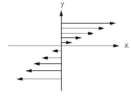
The physical picture of this dynamical system corresponds to the presence of a velocity flow field \({\textbf v}(y) = \gamma y\hat{\textbf x} \) shown in the figure.
The flow field points in the \(\hat{\textbf x} \) direction and increases with increasing \(y\)-value. Thus, layers of a fluid, for example, will slow past each other, creating an anisotropy in the system. From the conserved quantity, one can see that the momentum of a particle is the value of \( {{\textbf p}_i} \) plus the contribution from the field evaluated at the position of the particle
\[ {\textbf p}_i \rightarrow {\textbf p}_i + m_i {\textbf v}(y_i) \nonumber \]
Such an applied external shearing force will create an asymmetry in the internal pressure. In order to describe this asymmetry, we need an analog of the internal pressure that contains a dependence on specific spatial directions. Such a quantity is known as the pressure tensor and can be defined analogously to the isotropic pressure \(P\) that we encountered earlier in the course. Recall that an estimator for the pressure was
\[ p = {1 \over 3V}\sum_{i=1}^N\left[{{\textbf p}_i^2 \over m_i} + {\textbf r}_i\cdot {\textbf F}_i\right] \nonumber \]
and \( P = \langle p\rangle \) in equilibrium. Here, \(V\) is the volume of the system. By analogy, one can write down an estimator for the pressure tensor \( {p_{\alpha\beta} } \):
\[ p_{\alpha\beta} = {1 \over V}\sum_{i=1}^N\left[{({\textbf p}_i\cdot \hat {e}_{\alpha})({\textbf P}_i \cdot \hat {\textbf e}_{\beta}) \over m_i} + ({\textbf r}_i \cdot \hat {\textbf e}_{\alpha} )({\textbf F}_i\cdot\hat{\textbf e}_{\beta})\right] \nonumber \]
and
\[ P_{\alpha\beta} = \langle p_{\alpha\beta}\rangle \nonumber \]
where \( {\hat{\textbf e}_{\alpha} }\) is a unit vector in the \(\alpha \) direction, \( {\alpha=x,y,z } \). This (nine-component) pressure tensor gives information about spatial anisotropies in the system that give rise to off-diagonal pressure tensor components. The isotropic pressure can be recovered from
\[ P = {1 \over 3}\sum_{\alpha}P_{\alpha\alpha} \nonumber \]
which is just 1/3 of the trace of the pressure tensor. While most systems have diagonal pressure tensors due to spatial isotropy, the application of a shear force according to the above scheme gives rise to a nonzero value for the \(xy\) component of the pressure tensor \(P_{xy}\). In fact, \(P_{xy}\) is related to the velocity flow field by a relation of the form
\[ P_{xy} = -\eta {\partial v_x \over \partial y} = -\eta\gamma \nonumber \]
where the coefficient \( \eta\) is known as the shear viscosity and is an example of a transport coefficient. Solving for \( \eta\) we find
\[ \eta = -{P_{xy} \over \gamma} = -\lim_{t\rightarrow\infty}{\langle p_{xy}(t) \rangle \over \gamma} \nonumber \]
where \( \langle p_{xy}(t)\rangle \) is the nonequilibrium average of the pressure tensor estimator using the above dynamical equations of motion.
Let us apply the linear response formula to the calculation of the nonequilibrium average of the \(xy\) component of the pressure tensor. We make the following identifications:
\[ F_e(t) = 1\;\;\;\;\;{\bf C}_i({\rm x}) = \gamma y_i\hat{\textbf x}\;\;\;\;\;{\bf D}_i({\rm x}) = -\gamma p_{y_i}\hat{\textbf x} \nonumber \]
Thus, the dissipative flux \(j({\rm x}) \) becomes
\[\begin{align*} j({\rm x}) &= \sum_{i=1}^N\left[{\textbf C}_i\cdot {\textbf F}_i - {\textbf D}_i\cdot {{\textbf p}_i \over m_i}\right] \\[4pt] &= \sum_{i=1}^N\left[\gamma y_i({\textbf F}_i\cdot \hat{\textbf x}) + \gamma p_{y_i}{{\textbf p}_i\cdot \hat{\textbf x} \over m_i}\right] \\[4pt] &= \gamma\sum_{i=1}^N\left[{({\textbf p}_i\cdot \hat{\textbf y})({\textbf p}_i \cdot \hat {\textbf x}) \over m_i} + ({\textbf r}_i\cdot \hat{\textbf y})({\textbf F}_i\cdot \hat{\textbf x})\right] \\[4pt] &= \gamma V p_{xy} \end{align*}\]
According to the linear response formula,
\[ \langle p_{xy}(t) \rangle = \langle p_{xy}\rangle_0 -\beta\gamma V\int_0^t ds \langle p_{xy}(0) p_{xy}(t-s)\rangle_0 \nonumber \]
so that the shear viscosity becomes
\[ \eta = \lim_{t\rightarrow\infty}\left[-{\langle p_{xy}\rangle _0 \over \gamma } + \beta V \int_0^t ds \langle p_{xy}(0)p_{xy}(t)\rangle_0\right] \nonumber \]
Recall that \( \langle\cdots\rangle_0 \) means average of a canonical distribution with \( {\gamma = 0 } \). It is straightforward to show that \( \langle p_{xy}\rangle_0=0 \) for an equilibrium canonical distribution function. Finally, taking the limit that \(t \rightarrow \infty \) in the above expression gives the result
\[ \eta = {V \over kT}\int_0^{\infty}dt \langle p_{xy}(0) p_{xy}(t)\rangle_0 \nonumber \]
which is a relation between a transport coefficient, in this case, the shear viscosity coefficient, and the integral of an equilibrium time correlation function. Relations of this type are known as Green-Kubo relations. Thus, we have expressed a new kind of thermodynamic quantity to an equilibrium time correlation function, which, in this case, is an autocorrelation function of the \(xy\) component of the pressure tensor.