
2.3: Computational Instructions
- Page ID
- 470356

\( \newcommand{\vecs}[1]{\overset { \scriptstyle \rightharpoonup} {\mathbf{#1}} } \)
\( \newcommand{\vecd}[1]{\overset{-\!-\!\rightharpoonup}{\vphantom{a}\smash {#1}}} \)
\( \newcommand{\id}{\mathrm{id}}\) \( \newcommand{\Span}{\mathrm{span}}\)
( \newcommand{\kernel}{\mathrm{null}\,}\) \( \newcommand{\range}{\mathrm{range}\,}\)
\( \newcommand{\RealPart}{\mathrm{Re}}\) \( \newcommand{\ImaginaryPart}{\mathrm{Im}}\)
\( \newcommand{\Argument}{\mathrm{Arg}}\) \( \newcommand{\norm}[1]{\| #1 \|}\)
\( \newcommand{\inner}[2]{\langle #1, #2 \rangle}\)
\( \newcommand{\Span}{\mathrm{span}}\)
\( \newcommand{\id}{\mathrm{id}}\)
\( \newcommand{\Span}{\mathrm{span}}\)
\( \newcommand{\kernel}{\mathrm{null}\,}\)
\( \newcommand{\range}{\mathrm{range}\,}\)
\( \newcommand{\RealPart}{\mathrm{Re}}\)
\( \newcommand{\ImaginaryPart}{\mathrm{Im}}\)
\( \newcommand{\Argument}{\mathrm{Arg}}\)
\( \newcommand{\norm}[1]{\| #1 \|}\)
\( \newcommand{\inner}[2]{\langle #1, #2 \rangle}\)
\( \newcommand{\Span}{\mathrm{span}}\) \( \newcommand{\AA}{\unicode[.8,0]{x212B}}\)
\( \newcommand{\vectorA}[1]{\vec{#1}} % arrow\)
\( \newcommand{\vectorAt}[1]{\vec{\text{#1}}} % arrow\)
\( \newcommand{\vectorB}[1]{\overset { \scriptstyle \rightharpoonup} {\mathbf{#1}} } \)
\( \newcommand{\vectorC}[1]{\textbf{#1}} \)
\( \newcommand{\vectorD}[1]{\overrightarrow{#1}} \)
\( \newcommand{\vectorDt}[1]{\overrightarrow{\text{#1}}} \)
\( \newcommand{\vectE}[1]{\overset{-\!-\!\rightharpoonup}{\vphantom{a}\smash{\mathbf {#1}}}} \)
\( \newcommand{\vecs}[1]{\overset { \scriptstyle \rightharpoonup} {\mathbf{#1}} } \)
\( \newcommand{\vecd}[1]{\overset{-\!-\!\rightharpoonup}{\vphantom{a}\smash {#1}}} \)
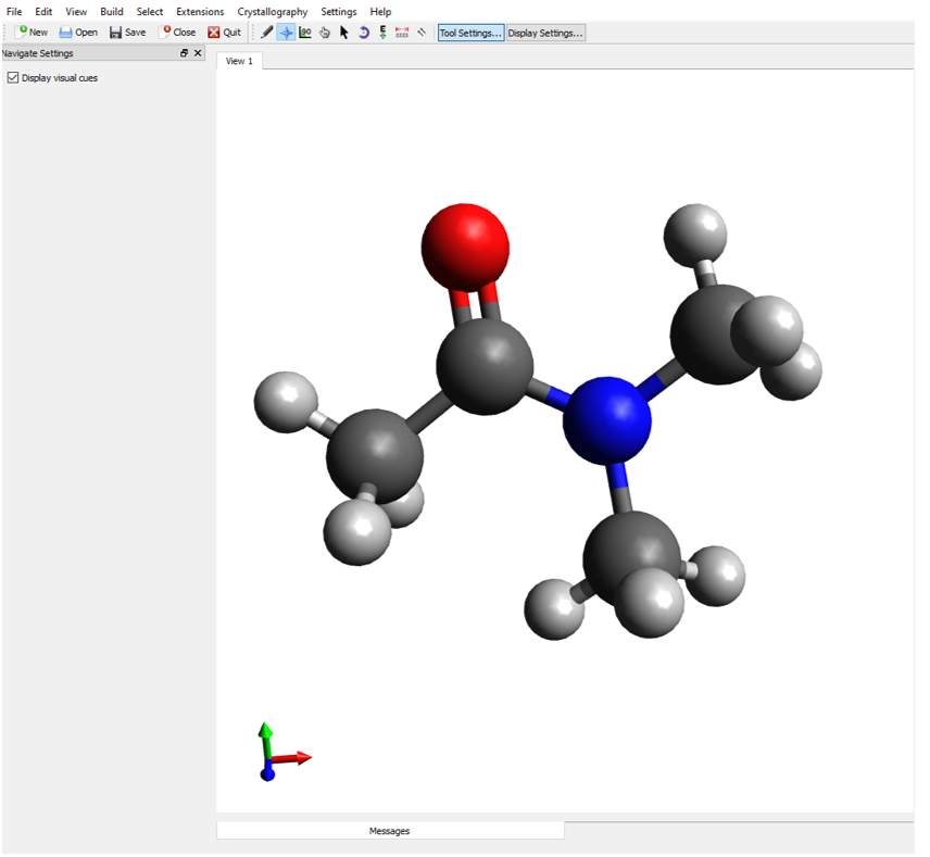
\(\newcommand{\avec}{\mathbf a}\) \(\newcommand{\bvec}{\mathbf b}\) \(\newcommand{\cvec}{\mathbf c}\) \(\newcommand{\dvec}{\mathbf d}\) \(\newcommand{\dtil}{\widetilde{\mathbf d}}\) \(\newcommand{\evec}{\mathbf e}\) \(\newcommand{\fvec}{\mathbf f}\) \(\newcommand{\nvec}{\mathbf n}\) \(\newcommand{\pvec}{\mathbf p}\) \(\newcommand{\qvec}{\mathbf q}\) \(\newcommand{\svec}{\mathbf s}\) \(\newcommand{\tvec}{\mathbf t}\) \(\newcommand{\uvec}{\mathbf u}\) \(\newcommand{\vvec}{\mathbf v}\) \(\newcommand{\wvec}{\mathbf w}\) \(\newcommand{\xvec}{\mathbf x}\) \(\newcommand{\yvec}{\mathbf y}\) \(\newcommand{\zvec}{\mathbf z}\) \(\newcommand{\rvec}{\mathbf r}\) \(\newcommand{\mvec}{\mathbf m}\) \(\newcommand{\zerovec}{\mathbf 0}\) \(\newcommand{\onevec}{\mathbf 1}\) \(\newcommand{\real}{\mathbb R}\) \(\newcommand{\twovec}[2]{\left[\begin{array}{r}#1 \\ #2 \end{array}\right]}\) \(\newcommand{\ctwovec}[2]{\left[\begin{array}{c}#1 \\ #2 \end{array}\right]}\) \(\newcommand{\threevec}[3]{\left[\begin{array}{r}#1 \\ #2 \\ #3 \end{array}\right]}\) \(\newcommand{\cthreevec}[3]{\left[\begin{array}{c}#1 \\ #2 \\ #3 \end{array}\right]}\) \(\newcommand{\fourvec}[4]{\left[\begin{array}{r}#1 \\ #2 \\ #3 \\ #4 \end{array}\right]}\) \(\newcommand{\cfourvec}[4]{\left[\begin{array}{c}#1 \\ #2 \\ #3 \\ #4 \end{array}\right]}\) \(\newcommand{\fivevec}[5]{\left[\begin{array}{r}#1 \\ #2 \\ #3 \\ #4 \\ #5 \\ \end{array}\right]}\) \(\newcommand{\cfivevec}[5]{\left[\begin{array}{c}#1 \\ #2 \\ #3 \\ #4 \\ #5 \\ \end{array}\right]}\) \(\newcommand{\mattwo}[4]{\left[\begin{array}{rr}#1 \amp #2 \\ #3 \amp #4 \\ \end{array}\right]}\) \(\newcommand{\laspan}[1]{\text{Span}\{#1\}}\) \(\newcommand{\bcal}{\cal B}\) \(\newcommand{\ccal}{\cal C}\) \(\newcommand{\scal}{\cal S}\) \(\newcommand{\wcal}{\cal W}\) \(\newcommand{\ecal}{\cal E}\) \(\newcommand{\coords}[2]{\left\{#1\right\}_{#2}}\) \(\newcommand{\gray}[1]{\color{gray}{#1}}\) \(\newcommand{\lgray}[1]{\color{lightgray}{#1}}\) \(\newcommand{\rank}{\operatorname{rank}}\) \(\newcommand{\row}{\text{Row}}\) \(\newcommand{\col}{\text{Col}}\) \(\renewcommand{\row}{\text{Row}}\) \(\newcommand{\nul}{\text{Nul}}\) \(\newcommand{\var}{\text{Var}}\) \(\newcommand{\corr}{\text{corr}}\) \(\newcommand{\len}[1]{\left|#1\right|}\) \(\newcommand{\bbar}{\overline{\bvec}}\) \(\newcommand{\bhat}{\widehat{\bvec}}\) \(\newcommand{\bperp}{\bvec^\perp}\) \(\newcommand{\xhat}{\widehat{\xvec}}\) \(\newcommand{\vhat}{\widehat{\vvec}}\) \(\newcommand{\uhat}{\widehat{\uvec}}\) \(\newcommand{\what}{\widehat{\wvec}}\) \(\newcommand{\Sighat}{\widehat{\Sigma}}\) \(\newcommand{\lt}{<}\) \(\newcommand{\gt}{>}\) \(\newcommand{\amp}{&}\) \(\definecolor{fillinmathshade}{gray}{0.9}\)Start by creating a folder on your desktop and naming it Resonance. Next, you should download the supplementary files associated with this exercise and move them to a folder that you just created. Contained within the supplementary files you will find a subfolder labeled DMA, which stands for dimethyl acetamide. Open DMA_coord.xyz in Avogadro to examine the structure of dimethyl acetamide. The starting structure of DMA should look like Figure 4 and show a functional group known as an amide, where a nitrogen is adjacent to a carbon-oxygen double bond. This file contains the input structure that we are going to tell our computational chemistry software package to optimize at the DFT level of theory.
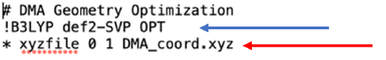
To optimize the structure of DMA we need to have an input file that tells Orca, the computational chemistry program that we are using, what we want to calculate and on what structure Orca should run the calculation. You can view this input file by clicking on DMA.inp within the DMA subfolder that you downloaded as part of the supplementary files. As shown in Figure 5, the input file is a brief text file with instructions for your computer. The first line of the input file, which starts with a number sign (#), is a comment indicating what the script is trying to accomplish. In this case, we are optimizing the geometry of DMA. The second line which begins with an exclamation point (!) tells Orca the functional of the calculation (B3LYP), the basis set (DEF2-SVP), and what we are asking the program to calculate (OPT-geometry optimization). Line 3, which beings with an asterisk (*), tells Orca what file contains the coordinate files for our molecule. The phrase xyzfile tells the computer that the file you are using has the molecule described using XYZ cartesian coordinates. There are then a series of two numbers which provide information about charge and spin of the chemical structure. The first number is the net charge of molecule(s) in the XYZ file. In this case it is zero because DMA is a neutral molecule. The second number is the net spin multiplicity (S) of the molecule that you are calculating, which in this case is 1 (singlet). We will talk more about the spin multiplicity of molecules in a later exercise, but for now you can think about this meaning that all electrons are paired so that they have a partner of the opposite spin. Finally, this line has the name of the coordinates file for DMA that we examined earlier.
Because Orca does not have a graphical user interface (GUI), we will need to tell the computer to run the calculation using the command prompt of the computer. To do this, right click the start button on your PC and search for the command prompt. First, we need to tell the computer to look on the C drive and we do this by typing C: and hitting enter in the command prompt. Next, we need to tell the computer where the input script and the coordinates file are to run the calculation. We do this by typing cd (space) and pasting the file path. When you hit enter, the computer will paste a new line indicating that the current directory has changed, as shown in Figure 6A. To find the file path of your input script, right click on the input script within the DMA subfolder and select properties. The file path will appear under location, and you can highlight and copy this file path as shown in Figure 6B.


Next, we will run the calculation by typing orca DMA.inp > DMA.out and pressing enter in the command prompt. At first, it may not appear like anything is happening, but the folder on your desktop labeled DMA will quickly become populated with the output of your calculation. Depending upon the speed of your computer, the calculation will take from 1-5 minutes, and upon completion the command prompt will print another line indicating that it is ready for the next command (Figure 7)

You can examine your results by opening the final geometry file DMA.xyz in Avogadro. To measure the bond lengths and angles, click on the measure button (looks like a ruler) and click on the atoms whose bond lengths and angles you want to measure (Figure 8).

References
- Hanwell, M. D.; Curtis, D. E.; Lonie, D. C.; Vandermeersch, T.; Zurek, E.; Hutchison, G. R. Avogadro: An Advanced Semantic Chemical Editor, Visualization, and Analysis Platform. J Cheminform 2012, 4 (1), 17. https://doi.org/10.1186/1758-2946-4-17.
- Avogadro: An Open-Source Molecular Builder and Visualization Tool. http://avogadro.cc/.
- Neese, F. The ORCA Program System. WIREs Computational Molecular Science 2012, 2 (1), 73–78. https://doi.org/10.1002/wcms.81.
- Neese, F. Software Update: The ORCA Program System, Version 4.0. WIREs Computational Molecular Science 2018, 8 (1), e1327. https://doi.org/10.1002/wcms.1327.
- Neese, F.; Wennmohs, F.; Becker, U.; Riplinger, C. The ORCA Quantum Chemistry Program Package. J. Chem. Phys. 2020, 152 (22), 224108. https://doi.org/10.1063/5.0004608.