4.5: Crystallinity in Polymers

We often think of polymers in the form of plastics: solid materials that serve some structural function, like a water bottle or some Venetian blinds. Polymers are different from many other such solids. Metals, for instance, have crystalline structures, in which atoms form a regularly repeating pattern, row upon row. Polymers, in contrast, are generally somewhat amorphous. Think of a strainer filled with cooked spaghetti, the long chains of pasta looping over each other randomly. That's how the molecules of amorphous or "shapeless" polymers tend to distribute themselves.

Polymers are capable of forming more ordered structures. If they aligned instead with their long chains parallel to each other, they would be able to get much closer together, and intermolecular attractions between the chains would be much stronger. The energy of the system would decrease, so this more crystalline structure should be inherently favored.

So why doesn't that always happen? Think about a polymer cooling from a completely melted state, in which case the structure is certainly amorphous. As it cools, the material becomes less like a liquid, and then less soft. With small molecules, that transition is relatively abrupt, as the molecules slide into place, guided by their strengthening intermolecular attractions. The molecules just have to rotate a little to face the correct direction, or maybe budge a little to the side. With polymers, the transition is much more gradual, because those great, long chains have to slide over each other and uncoil in order to lie parallel. At some point, there just isn't enough energy for them to keep working their way into the optimal alignment. As a result, many polymers are semi-crystalline, with regions called lamellae where portions of chains have aligned parallel to each other, but also with large amorphous areas that are much more randomly oriented.

As a result, a polymer sample might be 80% amorphous with only 20% of its chain lengths aligned in crystalline lamellae. Even so, those crystalline domains exert a strong influence on the properties of the polymer. Because of the stronger intermolecular attractions between these closer chains, the chains are much less able to slide past each other. The result is a material that is stronger and more rigid, and that can be very important for reliable structural materials.

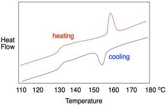
How do we know whether a polymer sample contains crystalline domains? We can use differential scanning calorimetry to observe the transition between an ordered crystalline phase and a disordered melt phase with added heat. As we saw when we were looking at glass transition, a melting point shows up as a peak on a DSC trace. You can look for it at a temperature above T_g, which you will recall looks more like a step in the baseline. Below T_g, the chains are not mobile enough to move out of alignment with each other. In the example below, you can see T_g at about 128 °C as well as a melting point, T_m, when attractions between chains in the lamellae are overcome, at 155-160 °C.

If this were a regular molecular or elemental solid, the melting point would be the same as the fusion point; the material would melt at the same temperature during warming as it froze during cooling. In polymers, it usually doesn't work out that way, and a hysteresis is observed. In hysteresis, a sample has changed because of previous events, leading to results that don't seem to be reproducible in the way that we would normally expect. In general, the crystallization temperature, T_c, is lower than the melting temperature, T_m. That's because, as the material melts, the chains move out of alignment with each other and, because of chain entanglement, they are hindered from getting back into alignment with each other again, leading to a delay in crystallization.

Example 4.5.1

Dec 31, 2019, 7:15 PM

Problem PP5.1.

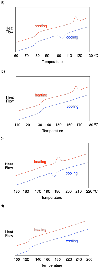
Describe what is observed in each of the following DSC traces.

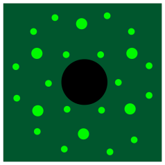
Crystallinity can also be probed in other ways. The classic approach is through X-ray diffraction. When X-rays pass through ordered materials, they give rise to diffraction patterns, bright spots in space where ricocheting X-rays have constructively interfered with each other, shining starkly amid the blackness where the X-rays have undergone destructive interference.

The drawing below is a cartoon of an X-ray diffraction pattern. It might be captured by a digital camera or, in earlier days, a sheet of photographic film. The bright spots result from X-rays scattering out from the middle, where they have encountered the sample. In the middle, the black circle blocks the original X-ray beam, which would otherwise be too bright to allow observation of those spots around it.

The data from an X-ray diffraction experiment is fed into a program that can mathematically deconvolute why the spots showed up where they did. The process has been compared to throwing a stone over your shoulder into a pond, then watching the ripples to decide where the stone must be. With one stone, that should be pretty easy. You would find the stone at the center of a circle of ripples. With two or more stones, interference patterns make the ripples more complex, and so it may take more work to determine where each stone lies in the pond.

The picture below illustrates the results of a relatively simple X-ray diffraction experiment commonly used with crystalline polymer samples. The technique is called wide-angle X-ray scattering, or WAXS. It simply reports the angle at which scattering intensity is observed relative to the initial X-ray beam. That angle corresponds to a distance between atoms in the sample, which in this case usually corresponds to a distance between parallel polymer chains. Sometimes there can be more than one peak, but this example is a simple one to start with.

The relationship between this scattering angle and an interatomic distance is given by Bragg's Law, a fundamental starting point in X-ray crystallography first expressed by Sir William Bragg and his son, Sir Lawrence Bragg. The law states that:

\[nλ = 2d\sin θ \label{bragg1}\]

in which n is an integer (typically assumed to be 1), lambda is the wavelength of the X-ray used (commonly 1.541 Å, although others are possible), d is the distance between regularly repeating atoms and θ is the scattering angle.

Rearranging Equation \ref{bragg1}, we find:

\[d = \dfrac{1.541}{2\sin θ}\]

In other words, the distance between atoms is inversely proportional to the scattering angle. The greater the angle, the smaller the distance.

Example 4.5.1

In each of the following cases, determine which sample (A or B) has a higher crystalline content.