4.2: Viscosity of Polymers

Polymers have come to occupy a very important niche in the materials we use every day. What makes them unique? Why do they have properties that aren't easily replicated by other materials?

Let's start with a property that you are probably familiar with. Viscosity is a term we use to describe the "thickness" of different liquids. For example, we say that honey is more viscous than water. Motor oil is more viscous than gasoline. When we say that, we mean that water is much easier to stir or to pour than honey. The honey moves more slowly. It resists the movement of the spoon when we stir it. Viscosity is often described in very general terms as "resistance to flow". The honey doesn't flow very easily, especially compared to something like water.

Now, honey isn't a polymer. It's a very concentrated solution. It contains a little bit of water and a whole lot of sugars, plus other small molecules produced by the plants from which the bees gathered the nectar to make the honey. The sugars aren't polymers, either; they are simple monosaccharides such as glucose and fructose. Nevertheless, this high viscosity is something honey has in common with polymer solutions, as well as with some oligomers, which are short-chain polymers that can be liquids instead of solids.

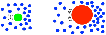
Why is honey so viscous? Partly it's just that the sugar molecules in the water are much larger than the water molecules, so they experience a lot more drag as they move through the solution compared to just plain water.

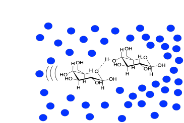
The strong intermolecular attractions between the individual sugar molecules are also a major factor. Sugars are covered in OH or hydroxyl groups that are capable of strong hydrogen bonds. As these molecules move past each other in the very concentrated solution, they cling to each other, slowing down the flow of the liquid.

The motor oil example works in a similar way. Motor oil and gasoline are composed of the same class of compounds, hydrocarbons, composed of carbon chains covered in hydrogen atoms. They're very similar to each other. The intermolecular attractions between the molecules are much weaker than those between sugar molecules; they're just London dispersion forces. The major difference between motor oil and gasoline is that the motor oil contains much longer hydrocarbon chains. The molecules are bigger, and so they experience more drag as they move through the liquid. The amount of intermolecular interactions is also crucial in determining how tightly two molecules hold onto each other, and this factor is especially important in very weak London dispersion forces, where a small advantage goes a long way. Those longer hydrocarbon chains in the motor oil cling to each other much more strongly than the shorter ones in the gasoline, so gasoline flows much more easily than motor oil.

For similar reasons, oligomers and polymers, if they are liquids, also display high viscosity. The extended contact between their long molecular chains leads to enhanced intermolecular attractions that contribute to a resistance to flow. Increased drag is also a factor; even in solution, these very large molecules encounter more resistance as they move past solvent molecules compared to the resistance smaller molecules would experience.

In fact, viscosity measurements of polymer solutions are another way to determine the size of the polymer -- leading to the chain length and the molecular weight. The larger the polymer, the more drag and also the more intermolecular attraction, and so the higher the viscosity.

So, the viscosity increases with the molecular weight, but not necessarily in a linear way. That can make it more difficult to use a graph like this to predict molecular weight from a viscosity measurement. One common thing to do in this situation is to take the log of the values. That approach will often give a straight line when two things are related.

Often in nature one physical property that depends on another will follow a "power law". That means that one quantity depends on the other raised to some exponent. In this case, the relationship is described by the Mark-Houwink equation:

\[ [η] = KM^α\]

In this equation, [η] is the intrinsic viscosity; that's the viscosity attributed to the solute, rather than the viscosity of the solvent itself. M is the molecular weight. K and α are constants for a particular polymer.

If you take the log of both sides of the equation -- that's OK to do mathematically, just like you could multiply both sides of an equation by four or subtract three from both sides and still have an equivalent expression -- you get:

\[\log[η] = log(KM^a)\]

If you take the log of two things multiplied together, it's the same as adding the individual logs of both things.

\[\log[η] = \log K + \log(M^a)\]

And if you take the log of something raised to an exponent, the exponent just comes down to become a coefficient.

\[\log[η] = \log K + α\log M\]

or

\[\log[η] = α \log M + \log K\]

That looks like an equation for a straight line:

\[y = mx + b.\]

Here, you plot \(\log[η]\) on the y axis, \(\log M\) on the x axis, and you get a straight line with those constants, \(α\) and \(K\), as the slope and y-intercept, respectively.

This approach does not yield an absolute measurement. You couldn't take two completely different polymers, take viscosity measurements, and make conclusions about which one had a higher average molecular weight. However, if you took a series of polymers of the same kind and measured their viscosities in solution, you would be able to deduce which ones were longer and which ones were shorter.

In fact, the dependence of viscosity on the molecular weight of polymers is more complicated than this graph suggests. If you deal with large enough polymers, the graph starts to look like this one:

Why does it bend? Remember, polymers in solution are coiled up into balls. A longer chain just corresponds to a bigger coil. At some point, these chains become big enough that they aren't likely to stay coiled independently of each other. They become more and more likely to interact with each other. They become entangled with each other.

There are plenty of other factors you would have to take into account in using viscosity to assess molecular weight. One of them is concentration, for example. The more concentrated a polymer solution, the more large molecules you have exerting drag and interacting with each other. Higher concentration leads to a higher viscosity measurement. Consequently, you would have to make sure you accounted for the polymer concentrations if you used this method.

Problem PP2.1.

Estimate the values of α and K for the polymer that provided the plot below.

Problem PP2.2.

Suppose you have a polymer described by the plot below. If your sample has a molecular weight of 1 million g/mol, what would you expect for intrinsic viscosity under the conditions of this experiment?

Problem PP2.3.

Suppose you have a calibration plot, below, for a particular polymer. If you measure the intrinsic viscosity of a sample and find that the value is 800 ml / g, what is the molecular weight of the sample?

Problem PP2.4.

Ethanol (CH₃CH₂OH) has an "absolute viscosity" of 1.095 centipoise, whereas ethylene glycol (HOCH₂CH₂OH) has an absolute viscosity of 16.2 centipoise. Explain why the two values are so different.