2.2: The Four Quantum Numbers
- Page ID
- 214180
\( \newcommand{\vecs}[1]{\overset { \scriptstyle \rightharpoonup} {\mathbf{#1}} } \)
\( \newcommand{\vecd}[1]{\overset{-\!-\!\rightharpoonup}{\vphantom{a}\smash {#1}}} \)
\( \newcommand{\id}{\mathrm{id}}\) \( \newcommand{\Span}{\mathrm{span}}\)
( \newcommand{\kernel}{\mathrm{null}\,}\) \( \newcommand{\range}{\mathrm{range}\,}\)
\( \newcommand{\RealPart}{\mathrm{Re}}\) \( \newcommand{\ImaginaryPart}{\mathrm{Im}}\)
\( \newcommand{\Argument}{\mathrm{Arg}}\) \( \newcommand{\norm}[1]{\| #1 \|}\)
\( \newcommand{\inner}[2]{\langle #1, #2 \rangle}\)
\( \newcommand{\Span}{\mathrm{span}}\)
\( \newcommand{\id}{\mathrm{id}}\)
\( \newcommand{\Span}{\mathrm{span}}\)
\( \newcommand{\kernel}{\mathrm{null}\,}\)
\( \newcommand{\range}{\mathrm{range}\,}\)
\( \newcommand{\RealPart}{\mathrm{Re}}\)
\( \newcommand{\ImaginaryPart}{\mathrm{Im}}\)
\( \newcommand{\Argument}{\mathrm{Arg}}\)
\( \newcommand{\norm}[1]{\| #1 \|}\)
\( \newcommand{\inner}[2]{\langle #1, #2 \rangle}\)
\( \newcommand{\Span}{\mathrm{span}}\) \( \newcommand{\AA}{\unicode[.8,0]{x212B}}\)
\( \newcommand{\vectorA}[1]{\vec{#1}} % arrow\)
\( \newcommand{\vectorAt}[1]{\vec{\text{#1}}} % arrow\)
\( \newcommand{\vectorB}[1]{\overset { \scriptstyle \rightharpoonup} {\mathbf{#1}} } \)
\( \newcommand{\vectorC}[1]{\textbf{#1}} \)
\( \newcommand{\vectorD}[1]{\overrightarrow{#1}} \)
\( \newcommand{\vectorDt}[1]{\overrightarrow{\text{#1}}} \)
\( \newcommand{\vectE}[1]{\overset{-\!-\!\rightharpoonup}{\vphantom{a}\smash{\mathbf {#1}}}} \)
\( \newcommand{\vecs}[1]{\overset { \scriptstyle \rightharpoonup} {\mathbf{#1}} } \)
\( \newcommand{\vecd}[1]{\overset{-\!-\!\rightharpoonup}{\vphantom{a}\smash {#1}}} \)
\(\newcommand{\avec}{\mathbf a}\) \(\newcommand{\bvec}{\mathbf b}\) \(\newcommand{\cvec}{\mathbf c}\) \(\newcommand{\dvec}{\mathbf d}\) \(\newcommand{\dtil}{\widetilde{\mathbf d}}\) \(\newcommand{\evec}{\mathbf e}\) \(\newcommand{\fvec}{\mathbf f}\) \(\newcommand{\nvec}{\mathbf n}\) \(\newcommand{\pvec}{\mathbf p}\) \(\newcommand{\qvec}{\mathbf q}\) \(\newcommand{\svec}{\mathbf s}\) \(\newcommand{\tvec}{\mathbf t}\) \(\newcommand{\uvec}{\mathbf u}\) \(\newcommand{\vvec}{\mathbf v}\) \(\newcommand{\wvec}{\mathbf w}\) \(\newcommand{\xvec}{\mathbf x}\) \(\newcommand{\yvec}{\mathbf y}\) \(\newcommand{\zvec}{\mathbf z}\) \(\newcommand{\rvec}{\mathbf r}\) \(\newcommand{\mvec}{\mathbf m}\) \(\newcommand{\zerovec}{\mathbf 0}\) \(\newcommand{\onevec}{\mathbf 1}\) \(\newcommand{\real}{\mathbb R}\) \(\newcommand{\twovec}[2]{\left[\begin{array}{r}#1 \\ #2 \end{array}\right]}\) \(\newcommand{\ctwovec}[2]{\left[\begin{array}{c}#1 \\ #2 \end{array}\right]}\) \(\newcommand{\threevec}[3]{\left[\begin{array}{r}#1 \\ #2 \\ #3 \end{array}\right]}\) \(\newcommand{\cthreevec}[3]{\left[\begin{array}{c}#1 \\ #2 \\ #3 \end{array}\right]}\) \(\newcommand{\fourvec}[4]{\left[\begin{array}{r}#1 \\ #2 \\ #3 \\ #4 \end{array}\right]}\) \(\newcommand{\cfourvec}[4]{\left[\begin{array}{c}#1 \\ #2 \\ #3 \\ #4 \end{array}\right]}\) \(\newcommand{\fivevec}[5]{\left[\begin{array}{r}#1 \\ #2 \\ #3 \\ #4 \\ #5 \\ \end{array}\right]}\) \(\newcommand{\cfivevec}[5]{\left[\begin{array}{c}#1 \\ #2 \\ #3 \\ #4 \\ #5 \\ \end{array}\right]}\) \(\newcommand{\mattwo}[4]{\left[\begin{array}{rr}#1 \amp #2 \\ #3 \amp #4 \\ \end{array}\right]}\) \(\newcommand{\laspan}[1]{\text{Span}\{#1\}}\) \(\newcommand{\bcal}{\cal B}\) \(\newcommand{\ccal}{\cal C}\) \(\newcommand{\scal}{\cal S}\) \(\newcommand{\wcal}{\cal W}\) \(\newcommand{\ecal}{\cal E}\) \(\newcommand{\coords}[2]{\left\{#1\right\}_{#2}}\) \(\newcommand{\gray}[1]{\color{gray}{#1}}\) \(\newcommand{\lgray}[1]{\color{lightgray}{#1}}\) \(\newcommand{\rank}{\operatorname{rank}}\) \(\newcommand{\row}{\text{Row}}\) \(\newcommand{\col}{\text{Col}}\) \(\renewcommand{\row}{\text{Row}}\) \(\newcommand{\nul}{\text{Nul}}\) \(\newcommand{\var}{\text{Var}}\) \(\newcommand{\corr}{\text{corr}}\) \(\newcommand{\len}[1]{\left|#1\right|}\) \(\newcommand{\bbar}{\overline{\bvec}}\) \(\newcommand{\bhat}{\widehat{\bvec}}\) \(\newcommand{\bperp}{\bvec^\perp}\) \(\newcommand{\xhat}{\widehat{\xvec}}\) \(\newcommand{\vhat}{\widehat{\vvec}}\) \(\newcommand{\uhat}{\widehat{\uvec}}\) \(\newcommand{\what}{\widehat{\wvec}}\) \(\newcommand{\Sighat}{\widehat{\Sigma}}\) \(\newcommand{\lt}{<}\) \(\newcommand{\gt}{>}\) \(\newcommand{\amp}{&}\) \(\definecolor{fillinmathshade}{gray}{0.9}\)The quantum numbers are parameters that describe the distribution of electrons in the atom, and therefore its fundamental nature. They are:
1. PRINCIPAL QUANTUM NUMBER (n) - Represents the main energy level, or shell, occupied by an electron. It is always a positive integer, that is n = 1, 2, 3 ...
2. SECONDARY QUANTUM NUMBER (l ) - Represents the energy sublevel, or type of orbital, occupied by the electron. The value of l depends on the value of n such that l = 0, 1, ... n-1. This number is sometimes also called azimuthal, or subsidiary.
3. MAGNETIC QUANTUM NUMBER (ml ) - Represents the number of possible orientations in 3-D space for each type of orbital. Since the type of orbital is determined by l, the value of ml ranges between -l and +l such that ml = -l, ...0, ...+l.
4. SPIN QUANTUM NUMBER (mS ) - Represents the two possible orientations that an electron can have in the presence of a magnetic field, or in relation to another electron occupying the same orbital. Only two electrons can occupy the same orbital, and they must have opposite spins. When this happens, the electrons are said to be paired. The allowed values for the spin quantum number ms are +1/2 and -1/2.
According to Heisenberg’s uncertainty principle, it is impossible to know the electron’s velocity and its position simultaneously. The exact position of the electron at any given time cannot be known. Therefore, it is impossible to obtain a photographic picture of the atom like we could of a busy street. Electrons are more like fast-moving mosquitoes in a swarm that cannot be photographed without appearing blurred. The uncertainty about their position persists even in the photograph. An alternative picture of the swarm can be obtained by describing the area where the mosquitoes tend to be concentrated and the factors that determine their preference for certain locations, and that’s the best we can do.
The quantum numbers provide us with a picture of the electronic arrangement in the atom relative to the nucleus. This arrangement is not given in terms of exact positions, like the photograph of a street, but rather in terms of probability distributions and potential energy levels, much like the mosquito swarm. The potential energy levels are described by the main quantum number n and by the secondary quantum number l. The probability distributions are given by the secondary quantum number l and by the magnetic quantum number ml .
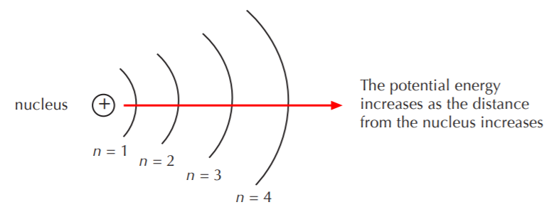
The now outdated solar system model of the atom allows us to visualize the meaning of the potential energy levels. The main energy levels, also called shells, are given by the main quantum number n.

THE RELATIONSHIP BETWEEN POTENTIAL ENERGY AND STABILITY IS INVERSE
As the potential energy of a system increases, the system’s stability is more easily disrupted. As an example consider the objects on the earth. Objects that are positioned at ground level have lower potential energy than objects placed at high altitudes. The object that’s placed at high altitude, be it a plane or a rock at the top of a mountain, has a higher “potential” to fall (lower stability) than the object that’s placed at ground level. Systems tend towards lower levels of potential energy, thus the tendency of the plane or the rock to fall. Conversely, an object placed in a hole on the ground does not have a tendency to “climb out” because its potential energy is even lower than the object placed at ground level. Systems do not naturally tend towards states of higher potential energy. Another way of saying the same thing is to say that systems tend towards states of higher stability.
In the case of the electrons in the atom, those at lower levels of potential energy (lower shells, or lower n) are more stable and less easily disrupted than those at higher levels of potential energy. Chemical reactions are fundamentally electron transfers between atoms. In a chemical reaction, it is the electrons in the outermost shell that react, that is to say, get transferred from one atom to another. That’s because they are the most easily disrupted, or the most available for reactions. The outermost shell is the marketplace where all electron trade takes place. Accordingly, it has a special name. It is called the valence shell.
Now, the solar system model of the atom is outmoded because it does not accurately depict the electronic distribution in the atom. Electrons do not revolve around the nucleus following elliptical, planar paths. They reside in 3-D regions of space of various shapes called orbitals.
An orbital is a region in 3-D space where there is a high probability of finding the electron.
An orbital is, so to speak, a house where the electron resides. Only two electrons can occupy an orbital, and they must do so with opposite spin quantum numbers ms . In other words, they must be paired.
The type and shape of orbital is given by the secondary quantum number l. As we know, this number has values that depend on n such that l = 0, 1, ... n-1. Furthermore, orbitals are not referred to by their numerical l values, but rather by small case letters associated with those values. Thus, when l = 0 we talk about s orbitals. When l = 1 we talk about p orbitals. When l = 2 we talk about d orbitals, and so on. In organic chemistry, we are mostly concerned with the elements of the second row and therefore will seldom refer to l values greater than 1. We’ll be talking mostly about s and p orbitals, and occasionally about d orbitals in reference to third row elements.
Since the value of l depends on the value of n, only certain types of orbitals are possible for each n, as follows (only the highest energy level is shown for each row of elements):

FIRST ROW ELEMENTS: n = 1 l = 0 only s orbitals are possible, denoted as 1s orbitals.
SECOND ROW ELEMENTS: n =2 l = 0 s orbitals are possible, denoted as 2s orbitals.
l = 1 p orbitals are possible, denoted as 2p orbitals.
THIRD ROW ELEMENTS: n = 3 l =0 s orbitals are possible, denoted as 3s orbitals
l =1 p orbitals are possible, denoted as 3p orbitals,
l =2 and d orbitals are possible, denoted as 3d orbitals.
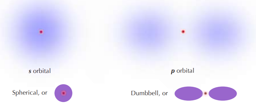
The shapes associated with s and p orbitals are shown below. For d orbitals refer to your general chemistry textbook. The red dot represents the nucleus.

Finally, the orientations of each orbital in 3-D space are given by the magnetic quantum number ml . This number depends on the value of l such that ml = -l, ...0, ...+l. Thus, when l = 0, ml = 0. There is only one value, or only one possible orientation in 3-D space for s-orbitals. That stands to reason, since they are spherical. In the case of p-orbitals l = 1, so ml = -1, 0, and +1. Therefore, there are three possible orientations in 3-D space for p-orbitals, namely along the x, y, and z axes of the Cartesian coordinate system. More specifically, those orbitals are designated as px, py, and pz respectively


