2.11: Intermolecular Forces and Relative Boiling Points (bp)

Learning Objective

• predict the relative boil points of organic compounds

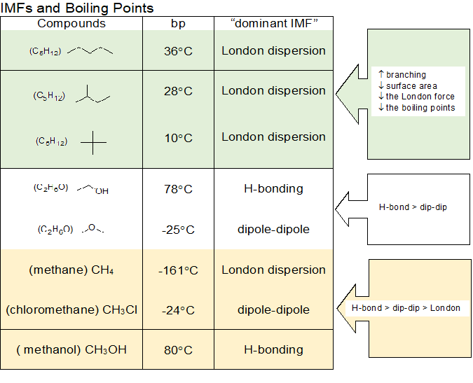
Intermolecular forces (IMFs) can be used to predict relative boiling points. The stronger the IMFs, the lower the vapor pressure of the substance and the higher the boiling point. Therefore, we can compare the relative strengths of the IMFs of the compounds to predict their relative boiling points.

H-bonding > dipole-dipole > London dispersion (van der Waals)

When comparing compounds with the same IMFs, we use size and shape as tie breakers since the London dispersion forces increase as the surface area increases. Since all compounds exhibit some level of London dispersion forces and compounds capable of H-bonding also exhibit dipole-dipole, we will use the phrase "dominant IMF" to communicate the IMF most responsible for the physical properties of the compound.

In the table below, we see examples of these relationships. When comparing the structural isomers of pentane (pentane, isopentane, and neopentane), they all have the same molecular formula C₅H₁₂. However, as the carbon chain is shortened to create the carbon branches found in isopentane and neopentane the overall surface area of the molecules decreases. The visual image of MO theory can be helpful in seeing each compound as a cloud of electrons in an all encompassing MO system. Branching creates more spherical shapes noting that the sphere allows the maximum volume with the least surface area. The structural isomers with the chemical formula C₂H₆O have different dominant IMFs. The H-bonding of ethanol results in a liquid for cocktails at room temperature, while the weaker dipole-dipole of the dimethylether results in a gas a room temperature. In the last example, we see the three IMFs compared directly to illustrate the relative strength IMFs to boiling points.

Boiling points and melting points

The observable melting and boiling points of different organic molecules provides an additional illustration of the effects of noncovalent interactions. The overarching principle involved is simple: the stronger the noncovalent interactions between molecules, the more energy that is required, in the form of heat, to break them apart. Higher melting and boiling points signify stronger noncovalent intermolecular forces.

Consider the boiling points of increasingly larger hydrocarbons. More carbons means a greater surface area possible for hydrophobic interaction, and thus higher boiling points.

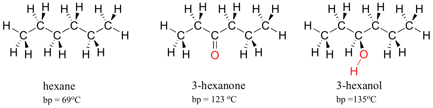
As you would expect, the strength of intermolecular hydrogen bonding and dipole-dipole interactions is reflected in higher boiling points. Just look at the trend for hexane (nonpolar London dispersion interactions only ), 3-hexanone (dipole-dipole interactions), and 3-hexanol (hydrogen bonding).

Of particular interest to biologists (and pretty much anything else that is alive in the universe) is the effect of hydrogen bonding in water. Because it is able to form tight networks of intermolecular hydrogen bonds, water remains in the liquid phase at temperatures up to 100 ^OC, (slightly lower at high altitude). The world would obviously be a very different place if water boiled at 30 ^OC.

Exercise

1. Based on their structures, rank phenol, benzene, benzaldehyde, and benzoic acid in terms of lowest to highest boiling point.

Solution

By thinking about noncovalent intermolecular interactions, we can also predict relative melting points. All of the same principles apply: stronger intermolecular interactions result in a higher melting point. Ionic compounds, as expected, usually have very high melting points due to the strength of ion-ion interactions (there are some ionic compounds, however, that are liquids at room temperature). The presence of polar and especially hydrogen-bonding groups on organic compounds generally leads to higher melting points. Molecular shape, and the ability of a molecule to pack tightly into a crystal lattice, has a very large effect on melting points. The flat shape of aromatic compounds such as napthalene and biphenyl allows them to stack together efficiently, and thus aromatics tend to have higher melting points compared to alkanes or alkenes with similar molecular weights.

Comparing the melting points of benzene and toluene, you can see that the extra methyl group on toluene disrupts the molecule's ability to stack, thus decreasing the cumulative strength of intermolecular London dispersion forces.

Note also that the boiling point for toluene is 111 ^oC, well above the boiling point of benzene (80 ^oC). The key factor for the boiling point trend in this case is size (toluene has one more carbon), whereas for the melting point trend, shape plays a much more important role. This makes sense when you consider that melting involves ‘unpacking’ the molecules from their ordered array, whereas boiling involves simply separating them from their already loose (liquid) association with each other.

If you are taking an organic lab course, you may have already learned that impurities in a crystalline substance will cause the observed melting point to be lower compared to a pure sample of the same substance. This is because impurities disrupt the ordered packing arrangement of the crystal, and make the cumulative intermolecular interactions weaker.

The melting behavior of lipid structures

An interesting biological example of the relationship between molecular structure and melting point is provided by the observable physical difference between animal fats like butter or lard, which are solid at room temperature, and vegetable oils, which are liquid. Both solid fats and liquid oils are based on a ‘triacylglycerol’ structure, where three hydrophobic hydrocarbon chains of varying length are attached to a glycerol backbone through an ester functional group (compare this structure to that of the membrane lipids discussed in section 2.4B).

Interactive 3D image of a saturated triacylglycerol (BioTopics)

Saturated vs mono-unsaturated fatty acid (BioTopics)

In vegetable oils, the hydrophobic chains are unsaturated, meaning that they contain one or more double bonds. Solid animal fat, in contrast, contains saturated hydrocarbon chains, with no double bonds. The double bonds in vegetable oils cause those hydrocarbon chains to be more rigid, and ‘bent’ at an angle (remember that rotation is restricted around double bonds), with the result that they don’t pack together as closely, and thus can be broken apart (ie. melted) more readily. Shown in the figure above is a polyunsaturated fatty acid chain (two double bonds), and you can click on the link to see interactive images of a saturated fatty acid compared to a monounsaturated fatty acid (one double bond).

Exercise

2. Arrange the following compounds in order of decreasing boiling point.

Answer

2.

Contributors

• William Reusch, Professor Emeritus (Michigan State U.), Virtual Textbook of Organic Chemistry

Organic Chemistry With a Biological Emphasis by Tim Soderberg (University of Minnesota, Morris)