6.9: Kinetics

Activation Energy

Since exothermic reactions are energetically (thermodynamically) favored, a careless thinker might conclude that all such reactions will proceed spontaneously to their products. Were this true, no life would exist on Earth, because the numerous carbon compounds that are present in and essential to all living organisms would spontaneously combust in the presence of oxygen to give carbon dioxide-a more stable carbon compound. The combustion of methane (eq.1), for example, does not occur spontaneously, but requires an initiating energy in the form of a spark or flame. The flaw in this careless reasoning is that we have focused only on the initial (reactant) and final (product) states of reactions. To understand why some reactions occur readily (almost spontaneously), whereas other reactions are slow, even to the point of being unobservable, we need to consider the intermediate stages of reactions.

Exothermic Single Step Reaction	Endothermic Single Step Reaction	Exothermic Two Step Reaction

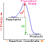
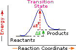
Every reaction in which bonds are broken will have a high energy transition state that must be reached before products can form. In order for the reactants to reach this transition state, energy must be supplied and reactant molecules must orient themselves in a suitable fashion. The energy needed to raise the reactants to the transition state energy level is called the activation energy, ΔE^‡. An example of a single-step exothermic reaction profile is shown on the left above, and a similar single-step profile for an endothermic reaction is in the center. The activation energy is drawn in red in each case, and the overall energy change (ΔE) is in green.
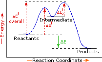
The profile becomes more complex when a multi-step reaction path is described. An example of a two-step reaction proceeding by way of a high energy intermediate is shown on the right above. Here there are two transition states, each with its own activation energy. The overall activation energy is the difference in energy between the reactant state and the highest energy transition state. We see now why the rate of a reaction may not correlate with its overall energy change. In the exothermic diagram on the left, a significant activation energy must be provided to initiate the reaction. Since the reaction is strongly exothermic, it will probably generate enough heat to keep going as long as reactants remain. The endothermic reaction in the center has a similar activation energy, but this will have to be supplied continuously for the reaction to proceed to completion.

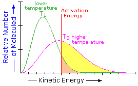
What is the source of the activation energy that enables a chemical reaction to occur? Often it is heat, as noted above in reference to the flame or spark that initiates methane combustion. At room temperature, indeed at any temperature above absolute zero, the molecules of a compound have a total energy that is a combination of translational (kinetic) energy, internal vibrational and rotational energies, as well as electronic and nuclear energies. The temperature of a system is a measure of the average kinetic energy of all the atoms and molecules present in the system. As shown in the following diagram, the average kinetic energy increases and the distribution of energies broadens as the temperature is raised from T₁ to T₂. Portions of this thermal or kinetic energy provide the activation energy for many reactions, the concentration of suitably activated reactant molecules increasing with temperature, e.g. orange area for T₁ and yellow plus orange for T₂. (Note that the area under a curve or a part of a curve is proportional to the number of molecules represented.)

Distribution of Molecular Kinetic Energy at Two Different Temperatures, T1 & T2

Reaction Rates and Kinetics

Chemical reactivity is the focus of chemistry, and the study of reaction rates provides essential information about this subject. Some reactions proceed so rapidly they seem to be instantaneous, whereas other reactions are so slow they are nearly unobservable. Most of the reactions described in this text take place in from 0.2 to 12 hours at 25 ºC. Temperature is important, since fast reactions may be slowed or stopped by cooling, and slow reactions are accelerated by heating. When a reaction occurs between two reactant species, it proceeds faster at higher concentrations of the reactants. These facts lead to the following general analysis of reaction rates.

Reaction Rate =	Number of Collisions between Reactant Molecules per Unit of Time	•	Fraction of Collisions with Sufficient Energy to pass the Transition State	•	an Orientational or Probability Factor

Since reacting molecules must collide to interact, and the necessary activation energy must come from the kinetic energy of the colliding molecules, the first two factors are obvious. The third (probability) factor incorporates the orientational requirements of the reaction. For example, the addition of bromine to a double bond at the end of a six-carbon chain (1-hexene) could only occur if the colliding molecules came together in a way that allowed the bromine molecule to interact with the pi-electrons of the double bond.
The collision frequency of reactant molecules will be proportional to their concentration in the reaction system. This aspect of a reaction rate may be incorporated in a rate equation, which may take several forms depending on the number of reactants. Three general examples are presented in the following table.

Reaction Type	Rate Equation	Reaction Order
A ——> B	Reaction Rate = k•[A]	First Order Reaction (no collision needed)
A + B ——> C + D	Reaction Rate = k•[A]*[B]	Second Order Reaction
A + A ——> D	Reaction Rate = k•[A]^2	Second Order Reaction

These rate equations take the form Reaction Rate = k[X] ⁿ[Y] ^m, where the proportionality constant k reflects the unique characteristics of a specific reaction, and is called the rate constant. The concentrations of reactants X and Y are [X] and [Y] respectively, and n & m are exponential numbers used to fit the rate equation to the experimental data. The sum n + m is termed the kinetic order of a reaction. The first example is a simple first order process. The next two examples are second order reactions, since n + m = 2. The kinetic order of a reaction is usually used to determine its molecularity.

In writing a rate equation we have disconnected the collision frequency term from the activation energy and probability factors defined above, which are necessarily incorporated in the rate constant k. This is demonstrated by the following equation.

The complex parameter A incorporates the probability factor. Because of the exponential relationship of k and the activation energy small changes in ΔE^‡ will cause relatively large changes in reaction rate. An increase in temperature clearly acts to increase k, but of greater importance is the increase in average molecular kinetic energy such an increase produces. This was illustrated in a previous diagram, increase in temperature from T₁ to T₂ producing a larger proportion of reactant molecules having energies equal or greater than the activation energy (designated by the red line.

Contributors

• William Reusch, Professor Emeritus (Michigan State U.), Virtual Textbook of Organic Chemistry