
8.4: Radiation measurements
- Page ID
- 372951

\( \newcommand{\vecs}[1]{\overset { \scriptstyle \rightharpoonup} {\mathbf{#1}} } \)
\( \newcommand{\vecd}[1]{\overset{-\!-\!\rightharpoonup}{\vphantom{a}\smash {#1}}} \)
\( \newcommand{\id}{\mathrm{id}}\) \( \newcommand{\Span}{\mathrm{span}}\)
( \newcommand{\kernel}{\mathrm{null}\,}\) \( \newcommand{\range}{\mathrm{range}\,}\)
\( \newcommand{\RealPart}{\mathrm{Re}}\) \( \newcommand{\ImaginaryPart}{\mathrm{Im}}\)
\( \newcommand{\Argument}{\mathrm{Arg}}\) \( \newcommand{\norm}[1]{\| #1 \|}\)
\( \newcommand{\inner}[2]{\langle #1, #2 \rangle}\)
\( \newcommand{\Span}{\mathrm{span}}\)
\( \newcommand{\id}{\mathrm{id}}\)
\( \newcommand{\Span}{\mathrm{span}}\)
\( \newcommand{\kernel}{\mathrm{null}\,}\)
\( \newcommand{\range}{\mathrm{range}\,}\)
\( \newcommand{\RealPart}{\mathrm{Re}}\)
\( \newcommand{\ImaginaryPart}{\mathrm{Im}}\)
\( \newcommand{\Argument}{\mathrm{Arg}}\)
\( \newcommand{\norm}[1]{\| #1 \|}\)
\( \newcommand{\inner}[2]{\langle #1, #2 \rangle}\)
\( \newcommand{\Span}{\mathrm{span}}\) \( \newcommand{\AA}{\unicode[.8,0]{x212B}}\)
\( \newcommand{\vectorA}[1]{\vec{#1}} % arrow\)
\( \newcommand{\vectorAt}[1]{\vec{\text{#1}}} % arrow\)
\( \newcommand{\vectorB}[1]{\overset { \scriptstyle \rightharpoonup} {\mathbf{#1}} } \)
\( \newcommand{\vectorC}[1]{\textbf{#1}} \)
\( \newcommand{\vectorD}[1]{\overrightarrow{#1}} \)
\( \newcommand{\vectorDt}[1]{\overrightarrow{\text{#1}}} \)
\( \newcommand{\vectE}[1]{\overset{-\!-\!\rightharpoonup}{\vphantom{a}\smash{\mathbf {#1}}}} \)
\( \newcommand{\vecs}[1]{\overset { \scriptstyle \rightharpoonup} {\mathbf{#1}} } \)
\( \newcommand{\vecd}[1]{\overset{-\!-\!\rightharpoonup}{\vphantom{a}\smash {#1}}} \)
\(\newcommand{\avec}{\mathbf a}\) \(\newcommand{\bvec}{\mathbf b}\) \(\newcommand{\cvec}{\mathbf c}\) \(\newcommand{\dvec}{\mathbf d}\) \(\newcommand{\dtil}{\widetilde{\mathbf d}}\) \(\newcommand{\evec}{\mathbf e}\) \(\newcommand{\fvec}{\mathbf f}\) \(\newcommand{\nvec}{\mathbf n}\) \(\newcommand{\pvec}{\mathbf p}\) \(\newcommand{\qvec}{\mathbf q}\) \(\newcommand{\svec}{\mathbf s}\) \(\newcommand{\tvec}{\mathbf t}\) \(\newcommand{\uvec}{\mathbf u}\) \(\newcommand{\vvec}{\mathbf v}\) \(\newcommand{\wvec}{\mathbf w}\) \(\newcommand{\xvec}{\mathbf x}\) \(\newcommand{\yvec}{\mathbf y}\) \(\newcommand{\zvec}{\mathbf z}\) \(\newcommand{\rvec}{\mathbf r}\) \(\newcommand{\mvec}{\mathbf m}\) \(\newcommand{\zerovec}{\mathbf 0}\) \(\newcommand{\onevec}{\mathbf 1}\) \(\newcommand{\real}{\mathbb R}\) \(\newcommand{\twovec}[2]{\left[\begin{array}{r}#1 \\ #2 \end{array}\right]}\) \(\newcommand{\ctwovec}[2]{\left[\begin{array}{c}#1 \\ #2 \end{array}\right]}\) \(\newcommand{\threevec}[3]{\left[\begin{array}{r}#1 \\ #2 \\ #3 \end{array}\right]}\) \(\newcommand{\cthreevec}[3]{\left[\begin{array}{c}#1 \\ #2 \\ #3 \end{array}\right]}\) \(\newcommand{\fourvec}[4]{\left[\begin{array}{r}#1 \\ #2 \\ #3 \\ #4 \end{array}\right]}\) \(\newcommand{\cfourvec}[4]{\left[\begin{array}{c}#1 \\ #2 \\ #3 \\ #4 \end{array}\right]}\) \(\newcommand{\fivevec}[5]{\left[\begin{array}{r}#1 \\ #2 \\ #3 \\ #4 \\ #5 \\ \end{array}\right]}\) \(\newcommand{\cfivevec}[5]{\left[\begin{array}{c}#1 \\ #2 \\ #3 \\ #4 \\ #5 \\ \end{array}\right]}\) \(\newcommand{\mattwo}[4]{\left[\begin{array}{rr}#1 \amp #2 \\ #3 \amp #4 \\ \end{array}\right]}\) \(\newcommand{\laspan}[1]{\text{Span}\{#1\}}\) \(\newcommand{\bcal}{\cal B}\) \(\newcommand{\ccal}{\cal C}\) \(\newcommand{\scal}{\cal S}\) \(\newcommand{\wcal}{\cal W}\) \(\newcommand{\ecal}{\cal E}\) \(\newcommand{\coords}[2]{\left\{#1\right\}_{#2}}\) \(\newcommand{\gray}[1]{\color{gray}{#1}}\) \(\newcommand{\lgray}[1]{\color{lightgray}{#1}}\) \(\newcommand{\rank}{\operatorname{rank}}\) \(\newcommand{\row}{\text{Row}}\) \(\newcommand{\col}{\text{Col}}\) \(\renewcommand{\row}{\text{Row}}\) \(\newcommand{\nul}{\text{Nul}}\) \(\newcommand{\var}{\text{Var}}\) \(\newcommand{\corr}{\text{corr}}\) \(\newcommand{\len}[1]{\left|#1\right|}\) \(\newcommand{\bbar}{\overline{\bvec}}\) \(\newcommand{\bhat}{\widehat{\bvec}}\) \(\newcommand{\bperp}{\bvec^\perp}\) \(\newcommand{\xhat}{\widehat{\xvec}}\) \(\newcommand{\vhat}{\widehat{\vvec}}\) \(\newcommand{\uhat}{\widehat{\uvec}}\) \(\newcommand{\what}{\widehat{\wvec}}\) \(\newcommand{\Sighat}{\widehat{\Sigma}}\) \(\newcommand{\lt}{<}\) \(\newcommand{\gt}{>}\) \(\newcommand{\amp}{&}\) \(\definecolor{fillinmathshade}{gray}{0.9}\)Radioactivity measurement
Radioactivity is measured in terms of the rate of radioactive events. Nuclear radiations are ionizing radiations, i.e., they knock off electrons from atoms or molecules that come in their path, leaving behind cations. Geiger Muller counter is one of the radiations measuring instruments that counts the disintegration of radionucleotide per second by registering the current produced by the ionization action of the radiation, as illustrated in Fig. 8.4.1. It is not just one ionization event; the nuclear particle keeps ionizing the atoms in its track until its energy is exhausted, as illustrated in Fig. 8.4.2. The instrument records the flash of electric current produced by the ionization of each radioactive disintegration.


The SI unit of radioactivity is Becquerel (Bq), i.e., the number of nuclei that disintegrate per second.
The common unit of radiation intensity is Curie (Ci), i.e., 3.7 x 10¹⁰ disintegrations per second. The relationship between Becquerel and Curie is the following.
\[1 \mathrm{Ci}=3.7 \times 10^{10} \mathrm{~Bq}=3.7 \times 10^{10} \text { disintegrations }\nonumber\]
Often the radioisotope for medical use has the information of millicurie per milliliter (mCi/mL) from which the volume for the desired dose can be calculated.
A patient must be given a 5.0 mCi dose of iodine-131 that is available as Na131I solution containing 3.8 mCi/mL. What volume of the solution should be administered?
Solution
Use the reciprocal of 3.8 mCi/mL as a conversion factor:
\[5.0 \cancel{\mathrm{~mCi}} \times \frac{1 \mathrm{~mL}}{3.8 \cancel{\mathrm{~mCi}}}=1.3 \mathrm{~mL} \text { dose }\nonumber\]
Radiation exposure measurements
Absorbed dose
The ionizing radiation dose or called the absorbed dose is measured in terms of energy deposited by ionizing radiation in a unit mass of matter being irradiated, as illustrated in Fig. 8.4.3
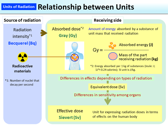
The SI unit of absorbed dose is gray (Gy) which is defined as the absorption of one joule of radiation energy per kilogram of matter (J/kg).
The common unit of absorbed dose is rad, which stands for radiation absorbed dose. The rad is one-hundredth of a gray, i.e.:
\[1 \mathrm{~Gy}=100 \mathrm{~rad}\nonumber\]
Equivalent dose
The same amount of energy deposited in tissues by different types of radiation carries different levels of health risks in terms of causing cancer and genetic damage, expressed as a radiation weighting factor (WR), as illustrated in Fig. 8.4.4, and listed in Fig. 8.4.5. For example, 1 Gy of \(\ce{beta}\)-particles carries a risk of 5.5% chances of eventually developing cancer, while 1 Gy of \(\ce{alpha}\)-particles has 20 times more risk compared to the β-particle (ref.: https://en.Wikipedia.org/wiki/Sievert, accessed on 07/15/2020). The health risk of the ionizing radiation is measured in the units of equivalent dose. Sievert (Sv) is an SI unit of an equivalent dose of ionizing radiation that measures the health effects of low levels of ionizing radiation on the human body.
The equivalent doze in Sievert (Sv) is equal to the product of absorbed dose in grays (Gy) multiplied the radiation weighting factor (WR), i.e., \(\text { The equivalent dose in } \mathrm{Sv}=\text { Absorbed dose in } \mathrm{Gy} \times \mathrm{W}_{\mathrm{R}}\)


The common unit of equivalent dose is rem (rem stands for roentgen equivalent man), which is:
\[1 \mathrm{~Sv}=100 \mathrm{rem}\nonumber\]
The personnel working in a radiation environment are required to wear film badges or electronic personal dosimeters, as shown in Fig. 8.4.6, that record the dose received. A record of each person's dose is usually maintained by the radiation facilities to comply with the allowed radiation exposure limits.

Effective dose
The equivalent dose is equal to the effective dose in sievert (Sv) when the whole human body is exposed equally to the radiation. If part of the body is exposed, then an effective dose in sievert (Sv) is calculated by the summation of the product of equivalent dose in Sv with tissue weighting factor (WT) for each tissue exposed to the radiation, as illustrated in Fig. 8.4.4 and calculated with example in Fig. 8.4.7. The reason for this calculation is that the effect of the same equivalent dose is different in different tissues. The tissue weighting factors (WT) are listed in Table 1.
An effective dose takes the absorbed dose and adjusts it for radiation type and organ sensitivity, i.e.,:
\[\text { The effective dose in } \mathrm{Sv}=\text { Equivalent dose in } \mathrm{Sv} \times \mathrm{W}_{\mathrm{T}}\nonumber\]

| Organs | WT |
|---|---|
| Gonads | 0.08 |
| Red bone marrow | 0.12 |
| Colon | 0.12 |
| Lung | 0.12 |
| Stomach | 0.12 |
| Breasts | 0.12 |
| Bladder | 0.04 |
| Liver | 0.04 |
| Oesophagus | 0.04 |
| Thyroid | 0.04 |
| Skin | 0.01 |
| Bone surface | 0.01 |
| Salivary glands | 0.01 |
| Brain | 0.01 |
| Remainder of body | 0.12 |
| Total | 1.00 |