Registration is now open for this year's LibreFest! Join us virtually the week of July 13.

6.9: VSEPR and Polarity

Last updated
Save as PDF

Page ID: 408819

$ \newcommand{\vecs}[1]{\overset { \scriptstyle \rightharpoonup} {\mathbf{#1}} } $

$ \newcommand{\vecd}[1]{\overset{-\!-\!\rightharpoonup}{\vphantom{a}\smash {#1}}} $

$ \newcommand{\dsum}{\displaystyle\sum\limits} $

$ \newcommand{\dint}{\displaystyle\int\limits} $

$ \newcommand{\dlim}{\displaystyle\lim\limits} $

$ \newcommand{\id}{\mathrm{id}}$ $ \newcommand{\Span}{\mathrm{span}}$

( \newcommand{\kernel}{\mathrm{null}\,}\) $ \newcommand{\range}{\mathrm{range}\,}$

$ \newcommand{\RealPart}{\mathrm{Re}}$ $ \newcommand{\ImaginaryPart}{\mathrm{Im}}$

$ \newcommand{\Argument}{\mathrm{Arg}}$ $ \newcommand{\norm}[1]{\| #1 \|}$

$ \newcommand{\inner}[2]{\langle #1, #2 \rangle}$

$ \newcommand{\Span}{\mathrm{span}}$

$ \newcommand{\id}{\mathrm{id}}$

$ \newcommand{\Span}{\mathrm{span}}$

$ \newcommand{\kernel}{\mathrm{null}\,}$

$ \newcommand{\range}{\mathrm{range}\,}$

$ \newcommand{\RealPart}{\mathrm{Re}}$

$ \newcommand{\ImaginaryPart}{\mathrm{Im}}$

$ \newcommand{\Argument}{\mathrm{Arg}}$

$ \newcommand{\norm}[1]{\| #1 \|}$

$ \newcommand{\inner}[2]{\langle #1, #2 \rangle}$

$ \newcommand{\Span}{\mathrm{span}}$ $ \newcommand{\AA}{\unicode[.8,0]{x212B}}$

$ \newcommand{\vectorA}[1]{\vec{#1}} % arrow$

$ \newcommand{\vectorAt}[1]{\vec{\text{#1}}} % arrow$

$ \newcommand{\vectorB}[1]{\overset { \scriptstyle \rightharpoonup} {\mathbf{#1}} } $

$ \newcommand{\vectorC}[1]{\textbf{#1}} $

$ \newcommand{\vectorD}[1]{\overrightarrow{#1}} $

$ \newcommand{\vectorDt}[1]{\overrightarrow{\text{#1}}} $

$ \newcommand{\vectE}[1]{\overset{-\!-\!\rightharpoonup}{\vphantom{a}\smash{\mathbf {#1}}}} $

$ \newcommand{\vecs}[1]{\overset { \scriptstyle \rightharpoonup} {\mathbf{#1}} } $

$\newcommand{\longvect}{\overrightarrow}$

$ \newcommand{\vecd}[1]{\overset{-\!-\!\rightharpoonup}{\vphantom{a}\smash {#1}}} $

$\newcommand{\avec}{\mathbf a}$ $\newcommand{\bvec}{\mathbf b}$ $\newcommand{\cvec}{\mathbf c}$ $\newcommand{\dvec}{\mathbf d}$ $\newcommand{\dtil}{\widetilde{\mathbf d}}$ $\newcommand{\evec}{\mathbf e}$ $\newcommand{\fvec}{\mathbf f}$ $\newcommand{\nvec}{\mathbf n}$ $\newcommand{\pvec}{\mathbf p}$ $\newcommand{\qvec}{\mathbf q}$ $\newcommand{\svec}{\mathbf s}$ $\newcommand{\tvec}{\mathbf t}$ $\newcommand{\uvec}{\mathbf u}$ $\newcommand{\vvec}{\mathbf v}$ $\newcommand{\wvec}{\mathbf w}$ $\newcommand{\xvec}{\mathbf x}$ $\newcommand{\yvec}{\mathbf y}$ $\newcommand{\zvec}{\mathbf z}$ $\newcommand{\rvec}{\mathbf r}$ $\newcommand{\mvec}{\mathbf m}$ $\newcommand{\zerovec}{\mathbf 0}$ $\newcommand{\onevec}{\mathbf 1}$ $\newcommand{\real}{\mathbb R}$ $\newcommand{\twovec}[2]{\left[\begin{array}{r}#1 \\ #2 \end{array}\right]}$ $\newcommand{\ctwovec}[2]{\left[\begin{array}{c}#1 \\ #2 \end{array}\right]}$ $\newcommand{\threevec}[3]{\left[\begin{array}{r}#1 \\ #2 \\ #3 \end{array}\right]}$ $\newcommand{\cthreevec}[3]{\left[\begin{array}{c}#1 \\ #2 \\ #3 \end{array}\right]}$ $\newcommand{\fourvec}[4]{\left[\begin{array}{r}#1 \\ #2 \\ #3 \\ #4 \end{array}\right]}$ $\newcommand{\cfourvec}[4]{\left[\begin{array}{c}#1 \\ #2 \\ #3 \\ #4 \end{array}\right]}$ $\newcommand{\fivevec}[5]{\left[\begin{array}{r}#1 \\ #2 \\ #3 \\ #4 \\ #5 \\ \end{array}\right]}$ $\newcommand{\cfivevec}[5]{\left[\begin{array}{c}#1 \\ #2 \\ #3 \\ #4 \\ #5 \\ \end{array}\right]}$ $\newcommand{\mattwo}[4]{\left[\begin{array}{rr}#1 \amp #2 \\ #3 \amp #4 \\ \end{array}\right]}$ $\newcommand{\laspan}[1]{\text{Span}\{#1\}}$ $\newcommand{\bcal}{\cal B}$ $\newcommand{\ccal}{\cal C}$ $\newcommand{\scal}{\cal S}$ $\newcommand{\wcal}{\cal W}$ $\newcommand{\ecal}{\cal E}$ $\newcommand{\coords}[2]{\left\{#1\right\}_{#2}}$ $\newcommand{\gray}[1]{\color{gray}{#1}}$ $\newcommand{\lgray}[1]{\color{lightgray}{#1}}$ $\newcommand{\rank}{\operatorname{rank}}$ $\newcommand{\row}{\text{Row}}$ $\newcommand{\col}{\text{Col}}$ $\renewcommand{\row}{\text{Row}}$ $\newcommand{\nul}{\text{Nul}}$ $\newcommand{\var}{\text{Var}}$ $\newcommand{\corr}{\text{corr}}$ $\newcommand{\len}[1]{\left|#1\right|}$ $\newcommand{\bbar}{\overline{\bvec}}$ $\newcommand{\bhat}{\widehat{\bvec}}$ $\newcommand{\bperp}{\bvec^\perp}$ $\newcommand{\xhat}{\widehat{\xvec}}$ $\newcommand{\vhat}{\widehat{\vvec}}$ $\newcommand{\uhat}{\widehat{\uvec}}$ $\newcommand{\what}{\widehat{\wvec}}$ $\newcommand{\Sighat}{\widehat{\Sigma}}$ $\newcommand{\lt}{<}$ $\newcommand{\gt}{>}$ $\newcommand{\amp}{&}$ $\definecolor{fillinmathshade}{gray}{0.9}$

VSEPR

Lewis dot structures are a great tool to visualize how electrons can be arranged in molecules. Further, drawing resonance structures and determining the formal charge can help us determine which structures are most stable. However, neither of these tools provide much insight into the physical configuration of a molecule in 3D space. For this, we turn to Valence Shell Electron Pair Repulsion theory, or VSEPR.

Once we draw a viable Lewis structure, we can use the following chart to translate the 2D representation to a 3D geometry:

VSEPR theory chart illustrating various molecular geometries with diagrams for linear, trigonal planar, tetrahedral, and more.

Chart courtesy of Boundless.com. License: CC BY-SA. This content is excluded from our Creative Commons license. For more information, see https://ocw.mit.edu/fairuse.

Example $\PageIndex{1}$

Draw Lewis dot diagrams and determine the 3D VSEPR geometry of the following molecules:

$\mathrm{CH}_4, \mathrm{NH}_3, \mathrm{H}_2 \mathrm{O}, \mathrm{SO}_3, \mathrm{SO}_2, \mathrm{CO}_2$

Solution

	Electrons around central atom	VESPR description	Sketch of 3D model
$\mathrm{CH}_4$	- 4 groups of electrons in bonds - 0 lone pairs	tetrahedral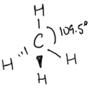
$\mathrm{NH}_3$	-3 groups of electrons in bonds -1 lone pair	trigonal pyramidal
$\mathrm{H}_2\mathrm{O}$	- 4 groups of electrons in bonds - 0 lone pairs	bent
$\mathrm{SO}_3$	- 4 groups of electrons in bonds - 0 lone pairs	trigonal planar
$\mathrm{SO}_2$	- 4 groups of electrons in bonds - 0 lone pairs	bent
$\mathrm{CO}_2$	- 4 groups of electrons - 0 lone pairs	linear	$A simple mathematical expression: $0 = c = 0$.$

Polarity

The difference in electronegativity across a molecule can generate electric dipole moments. Dipole moments are vector quantities, and by convention point from a more positive region of charge to a more negative region. If individual dipoles within a molecule cancel, there is no net dipole.

Example $\PageIndex{2}$

Determine whether $\mathrm{CO}_2$ and $\mathrm{H}_2\mathrm{O}$ have a net dipole moment.

Solution

Chemical structure diagram showing carbon dioxide (O=C=O) with electron movement arrows and charges.

In $\mathrm{CO}_2$, the two electronic dipoles are exactly opposite and cancel each other, so there isn’t a net dipole. Carbon dioxide is not a polar molecule.

Diagram of a water molecule (H₂O) showing bonds and partial charges (δ+, δ-).

In $\mathrm{H}_2\mathrm{O}$, the electronic dipoles don’t fully cancel, so there is a net dipole moment. Water is a polar molecule!

Search

Text Color

Text Size

Margin Size

Font Type

Example \(\PageIndex{1}\)

Solution

Example \(\PageIndex{2}\)

Solution

	Electrons around central atom	VESPR description	Sketch of 3D model
\(\mathrm{CH}_4\)	- 4 groups of electrons in bonds - 0 lone pairs	tetrahedral
\(\mathrm{NH}_3\)	-3 groups of electrons in bonds -1 lone pair	trigonal pyramidal
\(\mathrm{H}_2\mathrm{O}\)	- 4 groups of electrons in bonds - 0 lone pairs	bent
\(\mathrm{SO}_3\)	- 4 groups of electrons in bonds - 0 lone pairs	trigonal planar
\(\mathrm{SO}_2\)	- 4 groups of electrons in bonds - 0 lone pairs	bent
\(\mathrm{CO}_2\)	- 4 groups of electrons - 0 lone pairs	linear	$A simple mathematical expression: \(0 = c = 0\).$