
7.1: Bonding in Coordination Compounds
- Page ID
- 276167

\( \newcommand{\vecs}[1]{\overset { \scriptstyle \rightharpoonup} {\mathbf{#1}} } \)
\( \newcommand{\vecd}[1]{\overset{-\!-\!\rightharpoonup}{\vphantom{a}\smash {#1}}} \)
\( \newcommand{\id}{\mathrm{id}}\) \( \newcommand{\Span}{\mathrm{span}}\)
( \newcommand{\kernel}{\mathrm{null}\,}\) \( \newcommand{\range}{\mathrm{range}\,}\)
\( \newcommand{\RealPart}{\mathrm{Re}}\) \( \newcommand{\ImaginaryPart}{\mathrm{Im}}\)
\( \newcommand{\Argument}{\mathrm{Arg}}\) \( \newcommand{\norm}[1]{\| #1 \|}\)
\( \newcommand{\inner}[2]{\langle #1, #2 \rangle}\)
\( \newcommand{\Span}{\mathrm{span}}\)
\( \newcommand{\id}{\mathrm{id}}\)
\( \newcommand{\Span}{\mathrm{span}}\)
\( \newcommand{\kernel}{\mathrm{null}\,}\)
\( \newcommand{\range}{\mathrm{range}\,}\)
\( \newcommand{\RealPart}{\mathrm{Re}}\)
\( \newcommand{\ImaginaryPart}{\mathrm{Im}}\)
\( \newcommand{\Argument}{\mathrm{Arg}}\)
\( \newcommand{\norm}[1]{\| #1 \|}\)
\( \newcommand{\inner}[2]{\langle #1, #2 \rangle}\)
\( \newcommand{\Span}{\mathrm{span}}\) \( \newcommand{\AA}{\unicode[.8,0]{x212B}}\)
\( \newcommand{\vectorA}[1]{\vec{#1}} % arrow\)
\( \newcommand{\vectorAt}[1]{\vec{\text{#1}}} % arrow\)
\( \newcommand{\vectorB}[1]{\overset { \scriptstyle \rightharpoonup} {\mathbf{#1}} } \)
\( \newcommand{\vectorC}[1]{\textbf{#1}} \)
\( \newcommand{\vectorD}[1]{\overrightarrow{#1}} \)
\( \newcommand{\vectorDt}[1]{\overrightarrow{\text{#1}}} \)
\( \newcommand{\vectE}[1]{\overset{-\!-\!\rightharpoonup}{\vphantom{a}\smash{\mathbf {#1}}}} \)
\( \newcommand{\vecs}[1]{\overset { \scriptstyle \rightharpoonup} {\mathbf{#1}} } \)
\( \newcommand{\vecd}[1]{\overset{-\!-\!\rightharpoonup}{\vphantom{a}\smash {#1}}} \)
\(\newcommand{\avec}{\mathbf a}\) \(\newcommand{\bvec}{\mathbf b}\) \(\newcommand{\cvec}{\mathbf c}\) \(\newcommand{\dvec}{\mathbf d}\) \(\newcommand{\dtil}{\widetilde{\mathbf d}}\) \(\newcommand{\evec}{\mathbf e}\) \(\newcommand{\fvec}{\mathbf f}\) \(\newcommand{\nvec}{\mathbf n}\) \(\newcommand{\pvec}{\mathbf p}\) \(\newcommand{\qvec}{\mathbf q}\) \(\newcommand{\svec}{\mathbf s}\) \(\newcommand{\tvec}{\mathbf t}\) \(\newcommand{\uvec}{\mathbf u}\) \(\newcommand{\vvec}{\mathbf v}\) \(\newcommand{\wvec}{\mathbf w}\) \(\newcommand{\xvec}{\mathbf x}\) \(\newcommand{\yvec}{\mathbf y}\) \(\newcommand{\zvec}{\mathbf z}\) \(\newcommand{\rvec}{\mathbf r}\) \(\newcommand{\mvec}{\mathbf m}\) \(\newcommand{\zerovec}{\mathbf 0}\) \(\newcommand{\onevec}{\mathbf 1}\) \(\newcommand{\real}{\mathbb R}\) \(\newcommand{\twovec}[2]{\left[\begin{array}{r}#1 \\ #2 \end{array}\right]}\) \(\newcommand{\ctwovec}[2]{\left[\begin{array}{c}#1 \\ #2 \end{array}\right]}\) \(\newcommand{\threevec}[3]{\left[\begin{array}{r}#1 \\ #2 \\ #3 \end{array}\right]}\) \(\newcommand{\cthreevec}[3]{\left[\begin{array}{c}#1 \\ #2 \\ #3 \end{array}\right]}\) \(\newcommand{\fourvec}[4]{\left[\begin{array}{r}#1 \\ #2 \\ #3 \\ #4 \end{array}\right]}\) \(\newcommand{\cfourvec}[4]{\left[\begin{array}{c}#1 \\ #2 \\ #3 \\ #4 \end{array}\right]}\) \(\newcommand{\fivevec}[5]{\left[\begin{array}{r}#1 \\ #2 \\ #3 \\ #4 \\ #5 \\ \end{array}\right]}\) \(\newcommand{\cfivevec}[5]{\left[\begin{array}{c}#1 \\ #2 \\ #3 \\ #4 \\ #5 \\ \end{array}\right]}\) \(\newcommand{\mattwo}[4]{\left[\begin{array}{rr}#1 \amp #2 \\ #3 \amp #4 \\ \end{array}\right]}\) \(\newcommand{\laspan}[1]{\text{Span}\{#1\}}\) \(\newcommand{\bcal}{\cal B}\) \(\newcommand{\ccal}{\cal C}\) \(\newcommand{\scal}{\cal S}\) \(\newcommand{\wcal}{\cal W}\) \(\newcommand{\ecal}{\cal E}\) \(\newcommand{\coords}[2]{\left\{#1\right\}_{#2}}\) \(\newcommand{\gray}[1]{\color{gray}{#1}}\) \(\newcommand{\lgray}[1]{\color{lightgray}{#1}}\) \(\newcommand{\rank}{\operatorname{rank}}\) \(\newcommand{\row}{\text{Row}}\) \(\newcommand{\col}{\text{Col}}\) \(\renewcommand{\row}{\text{Row}}\) \(\newcommand{\nul}{\text{Nul}}\) \(\newcommand{\var}{\text{Var}}\) \(\newcommand{\corr}{\text{corr}}\) \(\newcommand{\len}[1]{\left|#1\right|}\) \(\newcommand{\bbar}{\overline{\bvec}}\) \(\newcommand{\bhat}{\widehat{\bvec}}\) \(\newcommand{\bperp}{\bvec^\perp}\) \(\newcommand{\xhat}{\widehat{\xvec}}\) \(\newcommand{\vhat}{\widehat{\vvec}}\) \(\newcommand{\uhat}{\widehat{\uvec}}\) \(\newcommand{\what}{\widehat{\wvec}}\) \(\newcommand{\Sighat}{\widehat{\Sigma}}\) \(\newcommand{\lt}{<}\) \(\newcommand{\gt}{>}\) \(\newcommand{\amp}{&}\) \(\definecolor{fillinmathshade}{gray}{0.9}\)Bonding in Coordination Compounds
This chapter is devoted to bonding theories for coordination compounds. Let us first think about, what a good theory should be able to do in general. The answer is, that it should be able to make many correct explanations for experimental observations based on a few, sensible, assumptions. In addition, it should be able to predict experimental observations. The more the theory can explain and predict, and the fewer the necessary assumptions, the better the theory. What does this mean for a bonding theory? What would a good bonding theory for coordination compounds be able to do? It should certainly be able to explain and predict the number of bonds and the shape of a molecule. In addition, it should be able to explain the magnetism of molecules, in particular dia- and paramagnetism. Remember, a molecule is diamagnetic when it has no unpaired electrons. It is paramagnetic when there are unpaired electrons. A diamagnetic molecule is repelled by an external magnetic field. A paramagnetic molecule is attracted by an external magnetic field. It should further be able to explain the stability and reactivity of complexes, as well as the optical properties of complexes. Optical properties of compounds are linked to bonding because they are related to electronic states.
Valence Bond Theory
There are essentially three bonding concepts that are used to describe the bonding in coordination compounds. The first one is the valence bond theory. The valence bond concept was introduced by Linus Pauling in 1931 to explain covalent bonding in molecules of main group elements.
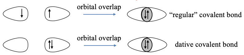
The basic idea is to overlap half-filled valence orbitals to form covalent bonds in which the two electrons are shared between the bonding partners (Fig. 7.1.1). These orbitals can either be atomic orbitals, or hybridized atomic orbitals. The concept works very well to explain the shapes of molecules of main group elements. The valence bond concept in its original form assumes that each bonding partner contributes one electron to the covalent bond. This is not consistent with the dative bonding in coordination compounds where it is assumed that one partner donates an electron pair and the other partner accepts it. To adapt valence bond theory to suit coordination compounds, Pauling suggested that a dative bond is formed via the overlap of a full valence orbital of the donor and an empty valence orbital of the acceptor. We will see that this concept can explain the shapes of coordination compounds in some cases, but overall it does not work very well. We will also see that valence bond theory can explain magnetism in some cases, but also here the valence bond theory has significant deficits. By its nature, valence bond theory cannot explain optical properties. Overall, valence bond theory is far more suitable for main group element molecules compared to transition metal complexes.
Crystal Field Theory
The second major theory is the crystal field theory. It is actually not a bonding theory because it is based on repulsive electrostatic interactions. It was originally developed to explain color in ionic crystals. Later, it was found that it can also explain colors in molecular coordination compounds, and is suitable to explain shapes and magnetism of complexes. However, because it is based on repulsive electrostatic interactions it cannot actually explain what holds the atoms in a molecule together. However, the crystal field theory is quite simple and convenient to use, and there is a lot of practicality to it.
Ligand Field Theory
The third theory is the ligand field theory. It is the most powerful theory, but also the most complicated one. Basically, it is molecular orbital theory applied to coordination compounds. It can make detailed statements about the number of bonds and shapes of molecules, and can explain the magnetism and optical properties of coordination compounds.
Valence Bond Theory for Coordination Compounds
Octahedral Complexes
Let us have a closer look at the valence bond theory, and assess valence bond theory for complexes by a number of examples.
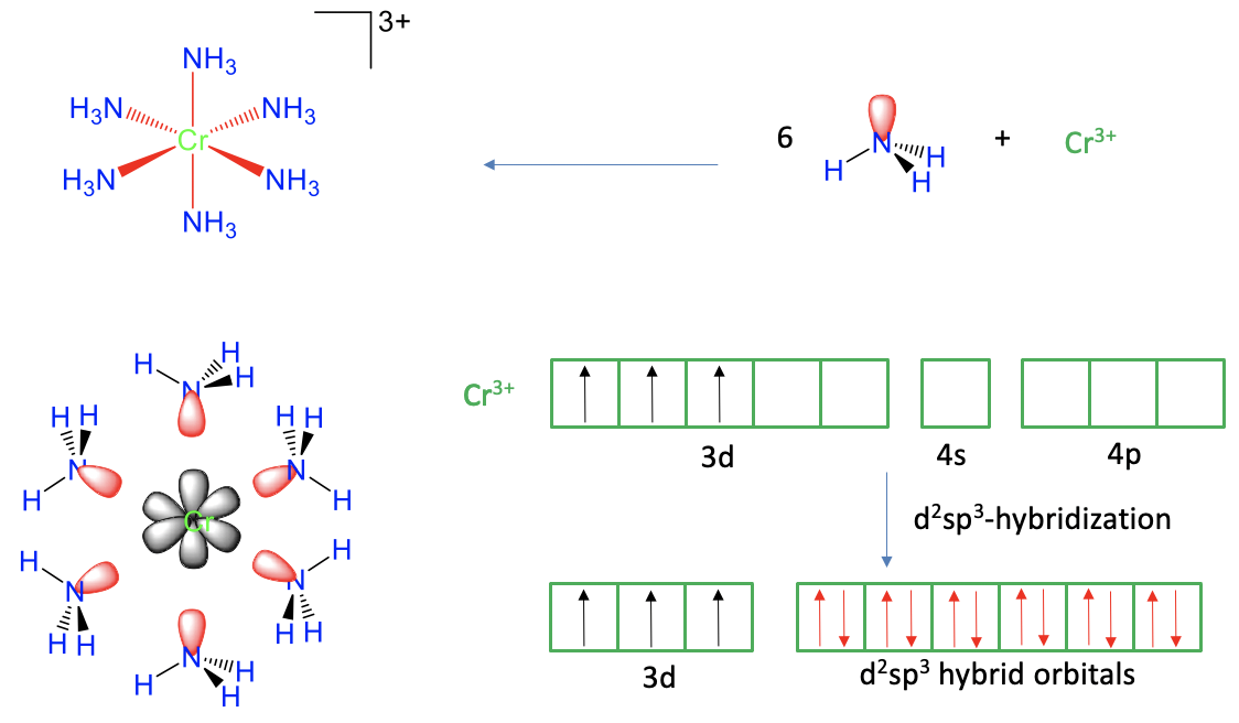 Figure 7.1.2 Valence bond theory applied to the hexaammine chromium (3+) cation
The first example is the hexaammine chromium (3+) cation (Fig. 7.1.2). From experiment we know that it has an octahedral shape, with six dative Cr-N bonds. Can valence bond theory explain the six bonds and the octahedral shape satisfactorily? In order to explain the six dative Cr-N bonds we would need to overlap six empty chromium valence orbitals with six filled valence orbitals of N. We can see that the six ammine ligands have one electron lone pair each that can serve as the valence orbitals. Does chromium have six empty valence orbitals? In order to assess this, we first need to know the oxidation state of the chromium. It is +3 because the ligands are all neutral when the bonds are cleaved heteroleptically, and the complex cation has a 3+ charge. Therefore, the chromium is a Cr3+ cation.
Next, we need to know the electron configuration of the Cr3+. A neutral Cr atom has the electron configuration 4s13d5. When a transition metal loses electrons to form a cation, it always loses its two valence electrons first, and then its d electrons. For chromium this means that we must remove the one 4s electron, and two of the five 3d-electrons. The three remaining 3d electrons are expected to be spin up in three different d orbitals according to Hund’s rule. How many empty valence orbitals remain? These would be two 3d and the 4s orbitals. In addition, it would also be justified to consider the three 4p orbitals as valence orbitals because the 4p orbitals are energetically only slightly higher than the 4s orbital. That means that we would have the six valence orbitals that we would need to explain the six bonds. There is, however, a complication. The six bonds in the complex are not distinguishable, but the six valance orbitals in the Cr3+ ion are distinguishable, for example, the 3d orbitals have different shape and energy than the 4s orbital, which is different from the 4p orbitals. Therefore, if we overlapped these orbitals with the electron lone pairs at N, the bonds would not be equivalent, or indistinguishable. We would have difficulty to explain the highly symmetric octahedral shape of the molecule. To go around this issue, valence bond theory uses the concept of hybridization. In this concept we mathematically mix the wave functions of the valence orbitals to form hybridized orbitals. In our example we would mix the two empty d-orbitals, the 4s orbital, and the three 4p orbitals to form six so-called d2sp3 hybridized orbitals. They have the same shape and size, and their lobes point toward the corners of an octahedron. Therefore, we can now create overlap between these six orbitals, and the six electron lone pairs at N to form six equivalent, indistinguishable Cr-N bonds. We conclude that we have now satisfactorily explained the bonding and the shape of the complex.
Can we also explain its magnetism? From experiment we know that the complex is paramagnetic, and that there are three unpaired electrons. Does valence bond theory predict the same? Yes, it does. There are three unpaired electrons in the three half-filled d-orbitals.
Tetrahedral Complexes
Our next is example is a tetrahedral complex, the tetrahydroxo zincate (2-) complex anion, Fig. 7.1.3.
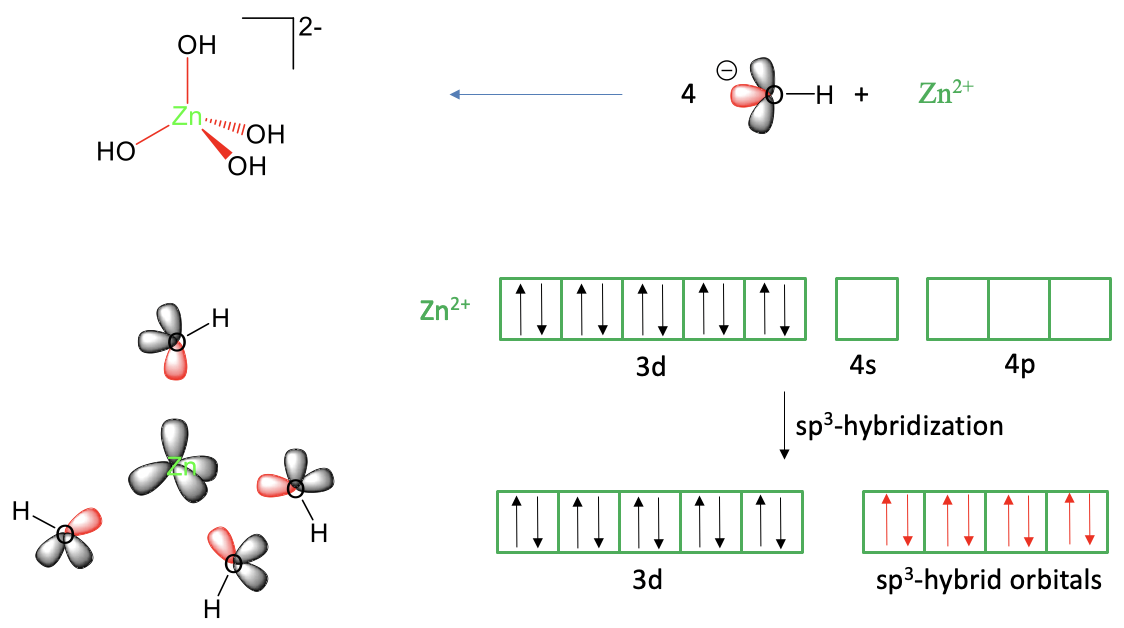
When viewing it as a Lewis-acid base complex with dative bonds it can be thought as an adduct of a Zn2+ and four hydroxide anions. One of the three electron lone pairs at the hydroxide ions would donate its electrons into empty Zn valence orbitals. That means we would need overall four empty Zn valence orbitals to explain the four Zn-O bonds. A neutral zinc atom has the electron configuration 4s2 3d10. We can derive this from the fact that zinc is in group 12 of period 4 in the periodic table. A Zn2+ ion has two electrons less. Because we must remove s electrons before we remove d electrons, the Zn2+ has the electron configuration 3d10. Like in the previous example we can justifiably consider the 4p orbitals as additional valence orbitals. We can see that we have four empty orbitals available to make the four bonds, namely the 4s and the 4p orbitals, but these orbitals are not equivalent, and do not have the correct orientation to explain the tetrahedral shape of the complex. There is a 90° angle between the p-orbitals which is smaller than the 109.5° tetrahedral bond angle in the molecule. However, we can solve this problem by hybridizing the 4s and the three 4p orbitals to form four sp3-hybridized orbitals. These hybrid orbitals have the property that their lobes point toward the corners of a tetrahedron. Thus, they are suitable to explain the tetrahedral shape of the molecule. We can place the ligands around the Zn2+ ion and approach the ligands on the bond axes to create orbital overlap between the empty sp3-hybridized orbitals and one electron lone pair at the oxygen atom. This produces the tetrahedral tetrahydroxo zincate (2-) anion.
Can we also explain the magnetism of the molecule? What magnetism would valence bond theory predict? We can see that there are no unpaired electrons in any of the metal valence orbitals. Thus, the complex should be diamagnetic. This is also what we find experimentally. Thus, valence bond theory is able to explain the magnetism of this complex anion.
Square Planar Complex
Now let us see if the valence bond theory can also explain a square planar complex such as tetracyanonickelate (2-).
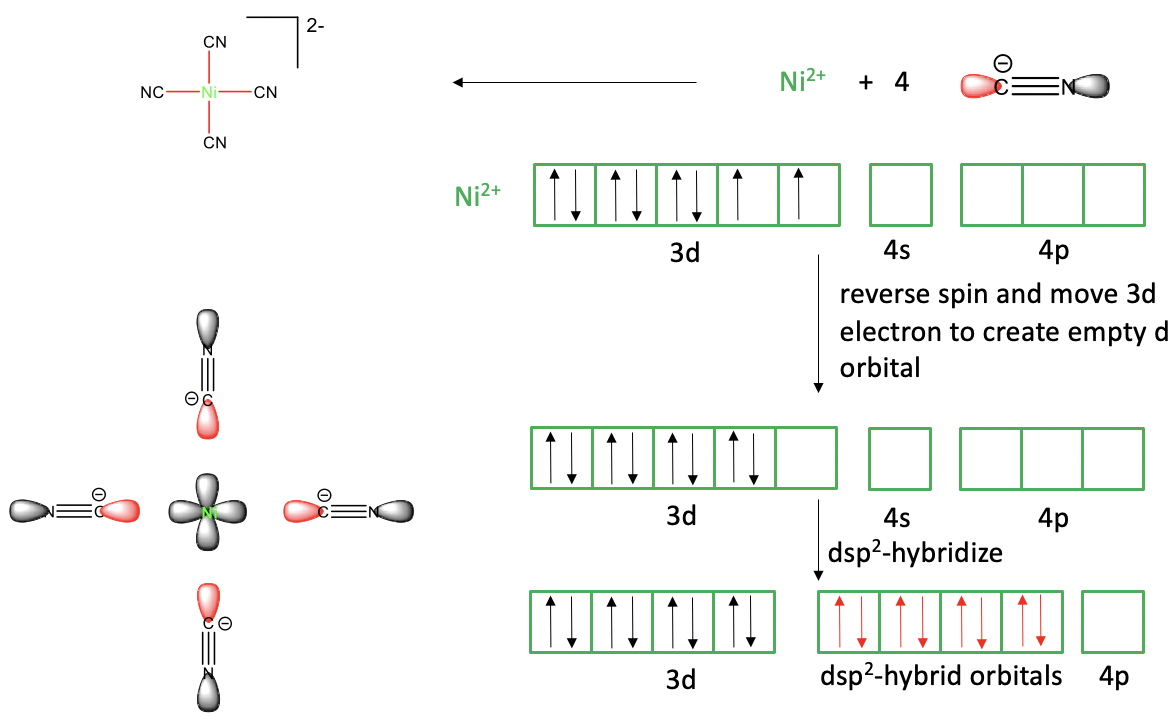 Figure 7.1.4 Valence bond theory applied to the tetracyanonickelate (2-) square planar complex
In the valence bond picture we view the Ni-CN bonds as dative bonds, and the complex is considered an adduct of Ni2+ and CN-. To explain the four bonds, the Ni2+ ion would need to have four empty valence orbitals. Ni is a group 10 metal and a neutral Ni atom has the electron configuration 4s23d8. To create a Ni2+ ion we must remove the two 4s electrons, and thus the Ni2+ has the electron configuration 3d8. Do we have four empty orbitals available? Yes, the 4s and the three 4p orbitals are empty but again they are not equivalent and thus not suitable to explain four equivalent Ni-C bonds. Can we hybridize these orbitals? Yes, we can, but the resulting four sp3 hybridized orbitals would not be suitable to explain the square planar shape, only the tetrahedral shape. What valence bond theory suggests in this case is to reverse the spin of one of the unpaired d electrons and move it into the other half-filled d-orbital. This produces an empty d-orbital that we can now hybridize with the 4s and two of the 2p orbitals to four dsp2-hybridized orbitals. These four orbitals have the property that their lobes point toward the vertices of a square, thus they are suitable to explain the square-planar shape. We can approach the ligands now on the bond axes to create orbital overlap between the empty dsp2 Ni and the electron lone pairs of the ligands. We can also say that the ligands donate their electron lone pairs into the hybridized metal orbitals. This produces the four covalent bonds that we need and yields a molecule of a square planar shape.
We can see that the valence bond theory can still explain the square planar shape, but only with the help of the additional assumption that one of the d-electrons gets spin-reversed and moves into another d-orbital. An assumption a theory makes should always be reasonable, so let us critique how reasonable this assumption is. Firstly, is the spin-reversal reasonable? Spin-reversal is a quantum-mechanically forbidden process, and thus it is questionable to assume that it happens. Secondly, there is no good explanation for why the electron moves. The energy of two spin-paired electrons in the same orbital is actually higher than that of two spin-paired electrons in different orbitals. So overall, we see that valence bond theory has difficulties to explain the square planar shape. It must make assumptions that are not very plausible.
Octahedral d5 High and Low Spin Orbital Complex
The valence bond theory has also difficulties to explain so-called high spin and low spin octahedral complexes. For example, it is known from magnetic measurements for 3d5 transition metal ions that they can make octahedral complexes with either one unpaired electron or five unpaired electrons, depending on the ligand. In the first case, the number of paired electrons in the d-orbitals is maximized, and we have a low-spin complex, in the other case the number of unpaired electrons is maximized, and we have a high spin complex. What approach does valence bond theory take to explain this phenomenon?
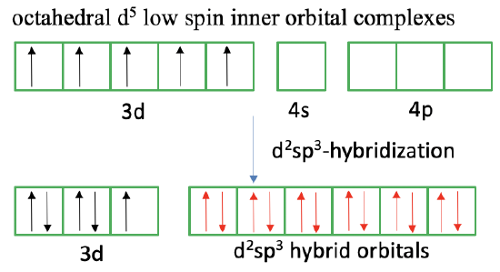
In the case of a low spin-complex, valence bond theory assumes a so-called inner orbital complex. Like in the square planar complex it is assumed that unpaired electrons reverse their spins and move into other half-filled d-orbitals so that spin-pairing is maximized. In the case of a d5 ion, two electrons reverse their spin, and move into two other half-filled orbitals. This leaves one unpaired electron. We see that due to the movement of the two electrons two 3d-orbitals are empty now, and so are the 4s and the 4p orbitals. The six empty orbitals can now be combined to form d2sp3-hybridized orbitals that can explain the octahedral shapes. Approaching the ligands overlaps the electron lone pair at the ligand with the empty hybrid orbitals to form a dative, covalent bond. We can also say the ligands donate electron lone pairs to form six covalent bonds. We can again criticize that spin-reversal is forbidden and spin-pairing is energetically unfavorable making the approach valence bond theory takes to explain the low-spin complex unsatisfactory.
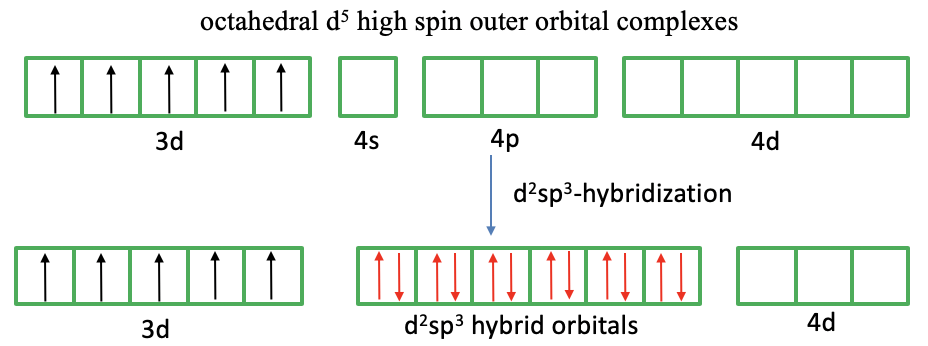
What about the 3d5 high spin complex (Fig. 7.1.6)? In this case we cannot pair spins to create empty d-orbitals because we need to explain five unpaired electrons. Now, valence bond theory makes another new assumption. It assumes that the outer 4d orbitals get involved in the bonding. These orbitals are empty and available for hybridization. We can therefore hybridize two 4d, the 4s, and the three 4p orbitals to form d2sp3 hybridized orbitals. In the last step we can approach the ligands, and the ligands can donate their electron lone pairs into the transition metal d-orbitals. Now we have explained the six bonds, the octahedral shape, and the five unpaired electrons.
We can again critique the valence bond approach. What justification is there to assume that the 4d orbitals are involved. The answer is: Very little. These orbitals are just too high in energy to be considered valence orbitals. It is not reasonable to assume that they are involved in the bonding. Therefore, again, we see that valence bond theory has difficulties to explain the properties of a complex. Valence bond theory also does not explain distortions of octahedral complexes due to the Jahn-Teller effect.
Octahedral d7 High and Low Spin Orbital Complex
High-spin and low-spin complexes are not only observed for octahedral complexes of d5-ions, but for example also for octahedral d7 ion complexes. A low-spin complex has three unpaired electrons and a high-spin complex has one unpaired electron. We will see that valence bond theory has even greater troubles to explain these compounds.
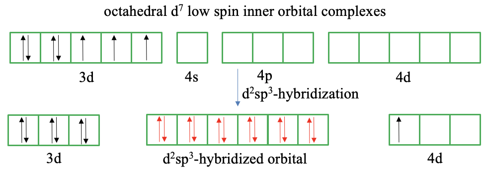
In a d7 ion there are four paired and three unpaired electrons according to Hund’s rule (Fig. 7.1.7). We can reverse the spin of one unpaired electron and pair it with an unpaired electron in another half-filled orbital to reduce the number of unpaired electrons to one. However, this gives us only one empty 3d orbital available for d2sp3-hybridization. In this case we cannot produce more empty 3d-orbitals by reversing the spin. Therefore, we must make again the questionable assumption that outer orbitals are involved in the bonding such as the 4d orbitals. Valence bond theory now suggests to move the unpaired electron from the 3d to the 4d orbital. This is simply done to create another empty 3d orbital that we need for d2sp3-hybridization. However, why would the 3d electron just go into another orbital of much higher energy? If we make this questionable assumption though, we have indeed six orbitals available for hybridization, and we can let the ligands donate an electron pair into the empty hybrid orbitals.
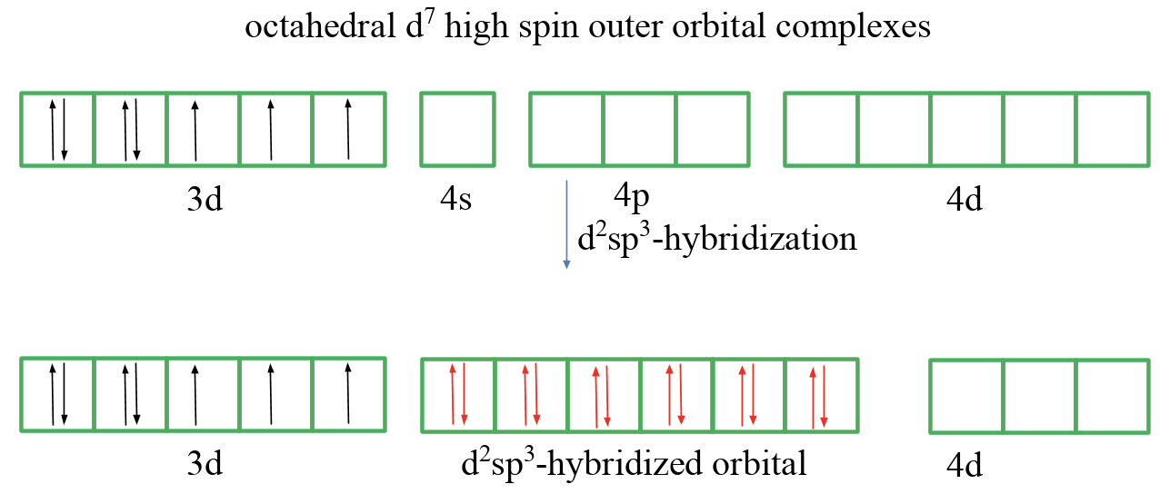
Finally, let us discuss an octahedral d7 high-spin outer orbital complex (Fig. 7.1.8). In this case we cannot pair any spins in the 3d orbitals. Therefore we assume again that the 4d orbitals get involved in the bonding, and hybridize two of them with the 4s and the three 4p orbitals. The six ligands can then donate six electron pairs into the orbitals thereby creating six bonds and explaining the octahedral shape.
Overall, we see that in the valence bond theory we move around electrons as we please in order to explain shapes and magnetism of complexes without good justification. Therefore, the valence bond theory, while extremely valuable for main group compounds, is only of limited use for transition metal complexes.
Crystal Field Theory
Now let us discuss the second bonding theory for coordination compounds, the crystal field theory. It is actually not a bonding theory because it is based on repulsive electrostatic interactions. Nonetheless, it has many features of a bonding theory in the sense that it can explain many phenomena that a bonding can explain, in particular molecular shape, magnetism, and optical properties.
What are the principles of crystal field theory? Crystal field theory assumes that the electrons in the metal d-orbitals are surrounded by an electric field which is caused by the ligand electrons. This electric field is called the crystal field. The name crystal field comes from the fact that this principle was first applied to transition metal ions surrounded by anions in crystals, and was only later extended to transition metal ions surrounded by ligands in molecular coordination compounds. The assumption that ligands surrounding a transition metal ion produce an electric field makes sense because the ligands contain electrons that are associated with an electric field. It is further assumed that the crystal field raises the energy of the metal-d-orbitals because of electrostatic repulsion between the ligand electrons and the metal electrons.
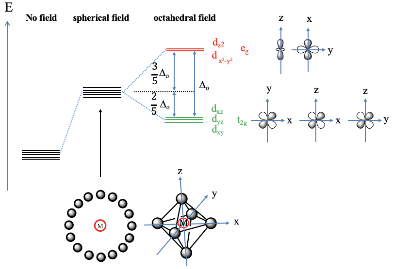
Let us first assume the hypothetical case that the ligand electrons surround the metal d-orbitals exactly spherically (Fig. 7.1.9, bottom left). In this case the electric field is completely isotropic, and this means that the energy of all five metal d-orbitals increases to the same extent. Now let us consider the practical case that the ligands surround the metal in octahedrally, which is the case in an octahedral complex. We can say we have an octahedral crystal field. The electric field will now not be spherical any more, it will be the strongest where the ligands are, namely on the vertices of the octahedron, and less strong elsewhere. The vertices of the octahedron lie on the x, y, and z axes of the coordinate system. Thus, the crystal field is the strongest on the axes, and less strong elsewhere. What consequence does this have on the metal d-orbital energies relative to the spherical crystal field? Orbitals that have their electron density mostly on the axes will experience a greater electrostatic repulsion from the crystal field, and therefore will be higher in energy. Orbitals that will have their electron density mostly elsewhere, meaning not on the axes, will experience smaller repulsion, and thus the energy will be smaller compared to the spherical crystal field. Which are the orbitals that have their electron density mostly on the axes? These are the dz2 and the dx2-y2 orbitals. The dz2 orbital has its energy density mostly on the z-axis, the dx2-y2 – orbital has its energy mostly on the x and the y axes. The energy of both orbitals is increased by exactly the same amount. This is not obvious given that the orbitals have very different shapes. To understand this, it helps to remember that when orbitals are symmetrically degenerate, they also must be energetically degenerate.
An octahedral complex belongs to the point group Oh and in the point group Oh the dz2 and the dx2-y2-orbitals are degenerate and have eg symmetry. Therefore, the dx2-y2 and the dz2-orbitals in an octahedral crystal field are also often just called the eg-orbitals. The remaining d-orbitals, the dxy, the dyz, and the dxz orbitals have their electron density mostly in between the axes, therefore their energy is lower compared to the spherical crystal field. The energy of all three orbitals is reduced by exactly the same amount. We can again understand this when considering that these orbitals are triple-degenerate in the point group Oh and have the symmetry type t2g. For that reason the dxy, the dyz, and the dxz in an octahedral crystal field are also often called the t2g-orbitals. The energy difference between the t2g and the eg orbitals is called Δo. The energy of the t2g orbitals is decreased by 2/5 Δo relative to the spherical crystal field, and the energy of the eg-orbitals is increased by 3/5 Δo relative to the spherical crystal field. Where do the factors 2/5 and 3/5 come from? They are due to the law of the conservation of energy. The overall energy reduction due to the energy decrease of the t2g-orbitals must be equal to the overall energy increase due to the energy increase of the eg orbitals: ΣE(t2g)=-Σ(E(eg). Because there are three t2g orbitals but only two eg orbitals this equation only holds when the energy of the eg orbitals is increased by 3/5 Δo and the energy of the t2g orbitals is decreased by 2/5Δo, or 3 x 2/5 Δo = 2 x 3/5 Δo. Note that the energy of all orbitals will be greater in comparison to the case of no electrical field existing, but the energy is increased to a greater extent for the eg-orbitals compared to the t2g orbitals.
The Tetrahedral Crystal Field
What about a tetrahedral complex with a tetrahedral crystal field?
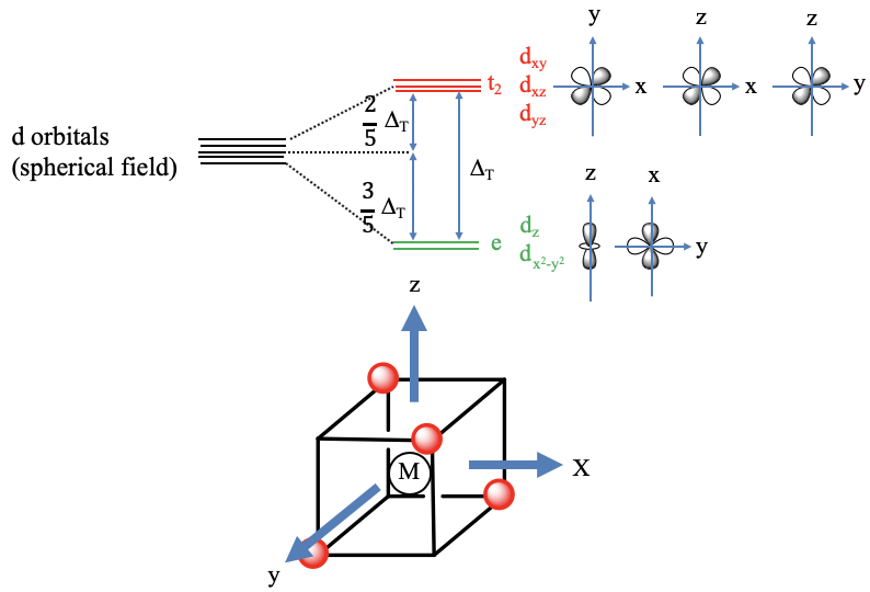
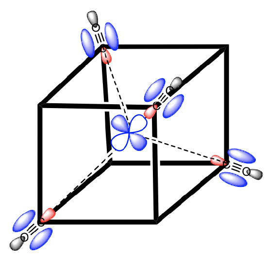
In this case, the ligands do not approach on the axes (Fig. 7.1.10). We can understand this when we consider that we can inscribe a tetrahedron in a cube. If we connect every other corner of a cube then we obtain a tetrahedron. We can define the coordinate system so that the three axes go through the centers of the square faces of the cube. We can see that the axes do not point toward the ligands, thus the ligands do not approach on the axes. Therefore, the orbitals that have their electron density mostly on the axes have a decreased energy relative to the spherical crystal field. These are the dz2 and the dx2-y2 orbitals. Their energy is the same despite the fact that they have quite different shape. We can explain this again with symmetry arguments. In the point group Td the dx2-y2 and the dz2 – orbitals are double-degenerate and have the symmetry type e. Because they are symmetrically degenerate, they are also energetically degenerate. The energy of the dxy, the dyz, and the dxz orbitals have most of their energy density in between the axes. Therefore, their energies are increased relative to the spherical crystal field. They are increased by the same amount because the orbitals are triply degenerated in the point group Td and have the symmetry type t2. The energy difference between the e and the t2 orbitals is called Δt. The energy of the t2 orbitals is decreased by 2/5 Δt. The energy of the e orbitals is increased by 3/5 Δt. This is again the due to the law of the conservation of energy. The total amount of decreased energy must equal the total amount of increased energy. The tetrahedral crystal field energy is smaller than that of the octahedral field because the octahedral field interacts more strongly with the d-orbitals compared to the tetrahedral field. One can calculate that it is actually just 4/9 of the octahedral field. This is mainly because the lobes of the t2 orbitals to not point exactly toward the vertices of the tetrahedron, while the lobes of the eg orbitals do point exactly toward the vertices of the octahedron.
Tetragonally Distorted Octahedral and Square Planar Crystal Fields
One nice feature of crystal field theory is that can can readily explain distortions such as the tetragonal distortion of octahedral complexes (Fig. 7.1.11).
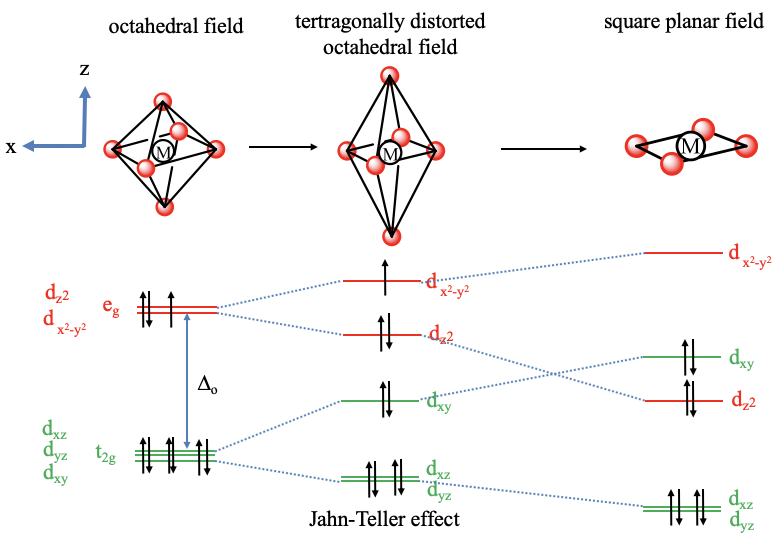
In a tetragonally distorted complex there is a tetragonally distorted crystal field. In an elongated octahedron two ligands are further away from the metal than the four others. Let us assume these two ligands are on the z-axis. Then, the crystal field is weaker on the z-axis. To keep the overall crystal field constant we must bring the other four ligands closer to the metal center. That means that we compress along the x and the y-axis. What will happen to the energy of the orbitals as the octahedron distorts? Because we elongate in the z-direction, the dz2 orbital, that has most electron density on the z-axis goes down in energy. Because we compress on the x and the y-axis, the energy of the dx2-y2 orbital increases. What about the t2g orbitals? The dxy orbital goes up in energy because it has electron density in the xy plane, but not along the z-axis. The dxz and dyz decrease in energy because they have a significant electron density in z-direction, and the electron density in z-direction is the same for both orbitals. We can now also think about, if the crystal field theory can explain why tetragonal distortion occurs preferentially for certain electron configurations of the metal. For example, it is known that metal ions with d9 electron configuration often make octahedral complexes with tetragonal distortions. For instance, the hexaaqua copper (2+) complex is an example of a tetragonally distorted complex with a Cu2+ ion that has a d9 electron configuration. We can understand that the tetragonal distortion occurs when comparing the energy of the electrons in the undistorted vs the distorted octahedron. In the undistorted octahedron we have three electrons in the degenerated eg orbitals. As we distort, we can move two electrons in the energetically lower dz2-orbital and fill the third one into the energetically higher dx2-y2-orbital. Thus, overall the electrons have a lower energy explaining the distortion. This is an example of the Jahn-Teller effect. In general, the Jahn-Teller effect can occur when there are partially occupied degenerate orbitals. In this case a molecule can lower its energy through distortion. Note that not only partial occupation of the eg-orbitals, but also partial occupation of the t2g-orbitals can cause the Jahn-Teller effect, although the effect is typically smaller. For example in complexes with metal ions the d4-electron configuration, all four electrons can be stabilized through Jahn-Teller distortion. It should also be noted that in addition to an elongation, there is also the possibility of compressing the octahedron along the z-axis. In this case the order of energy of the dz2 and the dx2-y2 orbital reverses, and the order of energy of the dxy, as well as the dxz and dyz reverses as well.
Finally, let us look at the square planar crystal field in square planar complexes. To understand the square planar crystal field it helps to understand the square planar shape as an infinitely elongated octahedron. If we move the two ligands along the z-axis infinitely far away from the metal ion, then we have created a square planar structure. How will the orbital energies change compared to an elongated octahedron? The dx2-y2 orbital will have an even higher energy due to the necessity to compensate for the decreased field associated with the ligands on the z-axis by further compressing along the x and the y-axis. The dz2-orbital is even further decreased in energy because the ligands along the z-axis are now completely gone. The dxy orbital is increased in energy because of the enhanced field in the xy-plane. It is now higher than the dz2-orbital. The dxz and the dyz orbitals are further decreased in energy because they have significant electron density in z-direction.
Viewing the square planar shape as an extreme case of a tetragonally elongated octahedron also lets us understand why the square planar shape is so often adopted by d8-metal complexes. We can see that the stabilization energy, and thus the tendency to distort is the greatest when two electrons are in the metal eg orbitals. In this case two electrons lower their energy through distortion and no electron has an increased energy. Thus, we would understand that the distortion becomes so great, so that the octahedral complex eventually loses two ligands and adopts the square planar shape. This is a nice example how crystal field theory can explain shapes and the number of bonds in a complex without actually being a bonding theory.
High Spin and Low Spin Complexes
One of the greatest strength of crystal field theory is that it can explain high-spin and low spin octahedral complexes in a simple way. The basis for that is the assumption that different ligands produce crystal fields of different strengths and that the differently strong crystal fields produce different Δo values. This assumption is plausible because it can be expected that different ligands interact differently with a metal ion, for example, the bond length or the bond strength may be different. If the ligands produce a large crystal field then we would expect a large Δo, when the crystal field is small, then we would expect a small Δo. The size of the Δo determines if we get a high spin or a low spin complex. If the Δo is larger than the spin pairing energy, then a low spin complex is favored, if Δo is smaller than the spin-pairing energy, then the high spin complex is favored.
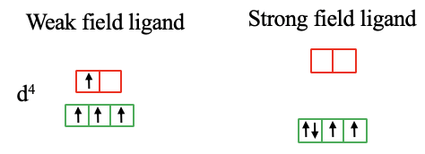
For example in a d4-metal complex with small Δo all electrons are unpaired (Fig. 7.1.12, left). Three of them are in the t2g-orbitals, and the fourth one is in the eg-orbital. Now let us assume a different ligand that can produce a Δo that is large enough to overcome the spin pairing energy. In this case the fourth electron would pair the spin of one of the three electrons in the t2g-orbitals (Fig. 7.1.12, right). We would obtain a low spin d4-complex.
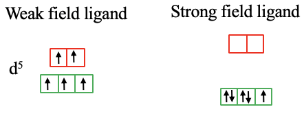
In the case of a d5-metal high spin complex there are five unpaired electrons, and all orbitals are half-filled. If the the ligand produces a crystal field large enough, the spin pairing energy is overcome and there are two paired and one unpaired electron in the t2g orbitals (Fig. 7.1.13).
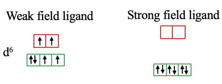
For a d6-metal high spin complex with a weak crystal field there are two unpaired electrons in the t2g and eg orbitals respectively. In the case of a strong field ligand and a low spin complex all electrons are in the t2g orbitals and all spins are paired (Fig. 7.1.14).
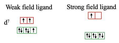
In the case of a d7-high spin complex there are two electron pairs and one unpaired electron in the t2g orbitals, and there are two unpaired electrons in the eg orbitals. For the low-spin complex the spin pairing energy is overcome. However, one electron must remain unpaired in the eg-orbitals because the t2g-orbitals are fully occupied with six electrons. The number of unpaired electrons in high and low spin complexes predicted by crystal field theory is what is experimentally observed. Therefore we can state that crystal field theory can quite elegantly explain high and low spin complexes.
We can also understand why there are no d1, d2, d3, d8, d9, and d10 low and high spin complexes. In the electron configurations d1-d3 all electrons are unpaired in the t2g orbitals. Therefore, there is no electron that could be moved from an eg to a t2g orbital. For the configurations d8-d10 all t2g orbitals are necessarily full. Therefore, there is no possibility to move an electron from an eg to a t2g orbital regardless the crystal field strength.
Further, we can explain why there are no low spin tetrahedral complexes. We have learned previously that a tetrahedral crystal field has only 4/9 of the strength of an octahedral field. Because it is so much weaker, no ligand is able to produce a field strong enough to overcome the spin pairing energy. High spin and low spin complexes are possible though for square planar complexes.
Strong and Weak Field Ligands: The Spectrochemical Series
Crystal field theory cannot only explain magnetism well, it can also make statements about the optical properties of a coordination compound. A complex can absorb light when an electron is excited from a d orbital of lower energy to a d orbital of higher energy. The larger the Δ, the smaller the wavelength of the absorbed light. In the case of an octahedral complex, absorption of light would excite an electron from a t2g to an eg orbital.
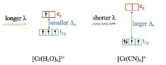
For example, an octahedral [Cr(H2O)]62+ complex has a smaller Δo compared to an octahedral [Cr(CN)6]4- complex (Fig. 7.1.16), and thus the aqua complex absorbs light of longer wavelength compared to the cyano complex. Vice versa, measuring the absorption spectrum of the complexes, allows us to make statements about the relative crystal field strength of the ligands. By measuring the absorption spectrum of many complexes with a variety of ligands we can develop a so-called spectrochemical series that orders ligands according to their field strength.
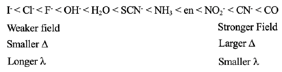
You can see such a series containing a non-exhaustive number of ligands in Fig. 7.1.17. You can see that the iodo ligands is on the very left side, and is the weakest field ligand, the carbonyl ligand is on the very right hand side, and is the strongest field ligand. All others are in between. We can see for example, that an aqua ligand is a stronger field ligand compared to a fluoro ligand, but a weaker ligand than an ammine ligand. Generally, ligands at the lower end of the series produce weaker fields, smaller Δs, and absorb light light with longer wavelengths. Ligands at the upper end of the series produce stronger fields, create larger Δs, and absorb light of shorter wavelengths. However, crystal filed theory cannot explain different ligand strength. Why does one ligand produce a stronger field than another? To answer this question, we need the ligand field theory.
Ligand Field Theory
Ligand field theory is the most powerful bonding theory for coordination compounds. It is essentially molecular orbital theory applied to coordination compounds. It can explain covalent bonding in coordination compounds, it can explain their shapes, it can explain their magnetism, and their electronic spectra. It can also explain the stability of coordination compounds, in particular the 18e rule and their exceptions. It is, however, more complicated than other bonding theories.
Just like in molecular orbital theory we can apply symmetry adapted linear combination of atomic orbitals to construct molecular orbitals. However, slightly modified rules apply to optimize molecular orbital theory for coordination compounds. These modifications are useful due to the greater complexity of coordination compounds. In the first step we determine the point group of the molecule and assign axes in a useful way. In the second step, we determine the valence orbitals, also called frontier orbitals of the metal. For example, for a transition metal of the 4th period we would consider the 4s, the 4p, and the 3d orbitals as the frontier orbitals. Next, we determine the symmetry of these orbitals. We can do this by just looking into the character table of the respective point group. In the following we select the highest-energy ligand orbitals that are suitable for σ-bonding. For ligands that are molecules or polyatomic ions, these orbitals are the HOMOs suitable for σ-bonding. For simple ions like chloro-ligands these are the highest occupied atomic orbitals. Next, we group the selected ligand orbitals to form ligand group orbitals (LGOs), and determine their symmetry types. To do so, we determine the reducible representation, and then the irreducible representations of the LGOs. This gives us the symmetry types of the ligand group orbitals. We then combine metal frontier orbitals and ligand group orbitals of the same symmetry type to form molecular orbitals. Now we have constructed all molecular orbitals suitable for σ-bonding, and can draw a molecular orbital diagram for the σ-bonding in the coordination compound.
Next, we look for ligand orbitals that are suitable for π-bonding with the metal. We then determine the symmetry types of their ligand group orbitals. Ligand group orbitals and metal orbitals of the same symmetry will then be combined to form molecular orbitals. These MOs represent the π-bonding in the molecule. We add these molecular orbitals to the molecular orbital diagram. Finally, we check if there are ligand orbitals suitable for \(\delta\)-bonding with the metal. If so, we also form ligands group orbitals for these, determine their symmetry types, and combine ligand group orbitals and metal orbitals of the same symmetry to form molecular orbitals. These orbitals will then also be added to the molecular orbital diagram.
Applicable rules for the construction of molecular orbital diagrams using ligand field theory
- Determine point group of the complex and assign axes.
- Determine which are the relevant metal frontier orbitals for bonding.
- Determine symmetry types of these metal orbitals.
- Select ligand HOMOs (suitable for σ-bonding) if the ligand is a molecule. If a simple ion, select the highest occupied atomic orbital.
- Form ligand group orbitals (LGOs) from selected ligand orbitals and determine their symmetry types.
- Combine metal orbitals and ligand group orbitals of appropriate symmetries to form molecular orbitals.
- Select ligand orbitals for \(π\) and \(σ\) bonding if applicable, determine their symmetry and combine them with appropriate metal orbitals.
Ligand Field Theory for an Octahedral Complex of a 4th Period Transition Metal
Let us apply the ligand field theory to a 4th period octahedral transition metal complex first. According to the rules we must first determine the point group and define the coordinate system. The point group is obviously Oh.
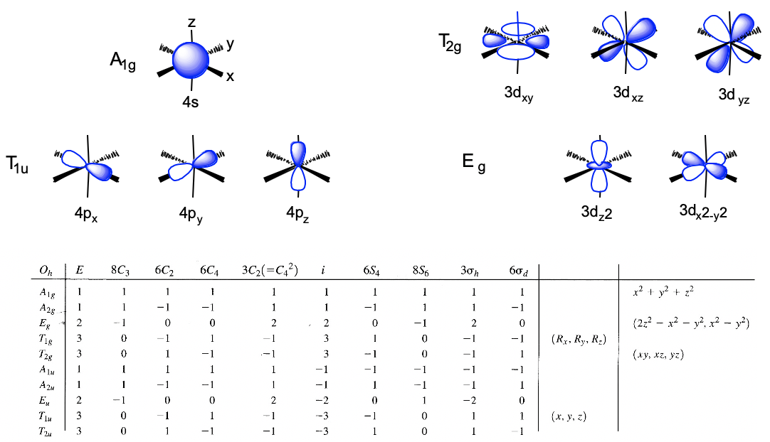
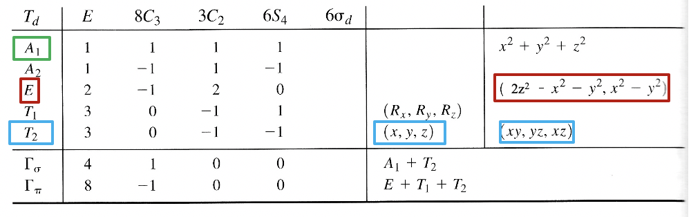
We can define the coordinate system so that the ligands approach on the x, y, and z axes, respectively. Next, we need to see what the frontier orbitals are. These would be the 4s, the 4p, and the 3d orbitals (Fig. 7.1.18). What symmetry types do they have? We can see this by looking into the character table for the point group Oh. An s orbital always has the totally symmetric symmetry type which is always listed first in the character table. In the point group Oh this is the symmetry type A1g. What about the 4p orbitals? We can see that the letters x,y, and z are in parentheses in the irreducible representation of the symmetry type T1u. This means that the three 4p orbitals are triply degenerate and have the symmetry type T1u. Finally, we need to determine the symmetry types of the 3d orbitals. We find xy, xz, and yz in parentheses in the irreducible representation of the symmetry type T2g. Thus, these orbitals have the symmetry type T2g. We further find 2z2-x2-y2 and x2-y2 in the line for the symmetry type Eg , thus the dz2 and the dx2-y2 orbitals are degenerate and have the symmetry type Eg. Remember here from the chapter about atomic structure that 2z2-x2-y2 mathematically describes a cone, and that the dz2 orbital has a conical node. We have now found all the symmetry types of the frontier orbitals.
Next, we need to direct our attention to the ligand and find the highest occupied molecular or atomic orbital suitable for σ-bonding. Of course, it depends now what the ligand is.
As an example let us choose the common and interesting carbonyl ligand (Fig. 7.1.19). To determine its HOMO suitable for σ-bonding with the metal, we will first need to know the molecular orbital diagram for the carbon monoxide molecule. The carbon monoxide molecule is a linear, polar molecule that belongs to the point group C∞v.
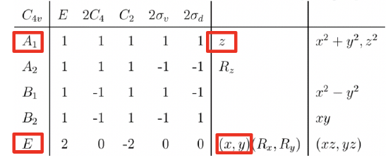
The character table of this point group is somewhat hard to work with because of the infinite order of the principal axis, and the infinite number of vertical mirror planes. We will therefore use the subgroup C4v instead (Fig. 7.1.20). A subgroup of a group is a group that results when we remove certain symmetry elements from the original group. We should remove symmetry elements so that degeneracies in the molecular orbitals are not overlooked, which can happen when you reduce the symmetry too much. The point group C4v is the point group with the lowest symmetry we can choose without overlooking degeneracies. Essentially, this is because the atomic orbitals of C and O are only 2s and 2p, and the 2p-orbitals perpendicular to the C-O bond axis can be rotated by 90° to make the orbitals interconvert. This requires a rotational axis of the order 4. If we chose the point group C2v, which has even lower symmetry, we would still be able to construct a molecular orbital diagram, but we would overlook that the 2px and the 2py orbitals are degenerate. We see that in the case of a diatomic linear molecule there is no central atom and no ligands. Therefore, we cannot apply the SALC method exactly as we previously learned it. Therefore, we treat the C and O atoms like central atom orbitals that interact with each other. To determine their symmetry types we can just look into the character table for C4v. We find that the 2s orbitals and the 2pz orbitals have the symmetry type A1 and the 2px and the 2py orbitals are double-degenerate and have the symmetry type E (Fig. 7.1.20). Now we can just combine the atomic orbitals to form molecular orbitals.
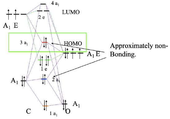
To construct a molecular orbital diagram we must consider that O is considerably more electronegative than C, and therefore, the 2s orbital of O is lower in energy compared to the 2s orbital of C. The 2p orbitals of O are lower in energy than those of C. Now we can label our orbitals with their symmetry types, and combine orbitals of the same symmetry type to form molecular orbitals (Fig. 7.1.21). We can start, for instance, with the orbitals of the A1 symmetry type. There are two on each side, so we will have overall four. Our qualitative assumption would be that there should be a strongly bonding and a strongly anti-bonding orbital, and weakly bonding and a weakly anti-bonding orbital in addition. The strongly bonding one would have the lowest energy and be labeled 1a1, the weakly bonding one would have higher energy and is labeled 2a1, the weakly anti-bonding one has an even higher energy and is labeled 3a1, and the strongly anti-bonding one would have the highest energy of all the four, and has the label 4a1. The strongly anti-bonding orbital must be above the 2pz orbital of C, and the strongly bonding one must be below the 2s orbital of O. We can write the 2a1 and the 3a1 orbital at energy levels so that the energy differences between all four a1 orbitals are about the same. We can now also connect the MOs and AOs of a1 symmetry with dotted lines. Now we can turn our attention to the orbitals with E symmetry. There are overall four orbitals of E symmetry, therefore, we expect two bonding double–degenerate orbitals with e-symmetry, and two anti-bonding double-degenerate orbitals with e-symmetry. The bonding MOs must be below the energy level of the 2p orbitals of O, and the two anti-bonding orbitals must be written above the energy levels of the 2p orbitals of C. We can now connect the atomic and molecular orbitals with dotted lines. Finally, we still need to fill in the electrons. There are four electrons coming from the carbon and six electrons coming from the oxygen, which gives ten electrons overall. This means that the 1a1, the 2a1, the 1e1 and the 3a1 molecular orbitals are full. This makes the 3a1 orbital the HOMO. It is suitable for σ-bonding with the metal because it has been created through σ-interactions between the 2pz and the 2s orbitals of O and P respectively.
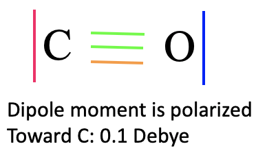
It is again interesting to compare the MO picture of the bonding in CO with the Lewis-dot structure (Fig. 7.1.19). In the Lewis dot structure we have a triple bond with six bonding electrons. They correspond to the bonding 1a1 and 1e electrons. In the Lewis dot structure all six electrons are energetically indistinguishable, but in the MO diagram we can clearly see that two electrons have a lower energy than the other four which are energetically degenerate. The 1a1 MO is a σ-orbital while the other two are π-orbitals because the 2px and the 2py orbitals interaction in π-fashion. The 2a1 and 3a1 orbitals can be approximated as non-bonding MOs representing the two electron lone pairs at C and O respectively. Because the 3a1 is slightly anti-bonding it has its electron density mostly at C, while the 2a1 is slightly bonding and therefore its counterpart is the electron lone pair at O. Interestingly the dipole moment of CO is slightly polarized toward C by 0.1 Debye despite the fact that O is the more electronegative atom. This can be attributed to the fact that the HOMO as a weakly anti-bonding orbital is primarily located at C, In addition, the 2a1 orbital is fairly close in energy to the 2s of C, therefore the 2s of C contributes significantly to this orbital. This leads to the fact that there is a significant amount of electron density located at C as well.
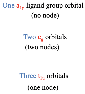
In the next step, we need to group the six HOMOs to form ligand group orbitals, and determine their symmetry types. This is being done by first determining the reducible representation of the orbitals using the orbital swapping method, and then determining the number of irreducible representations of a given type using the reduction formula from group theory. We will not go through the details of the calculations here, because there is nothing really new to learn, but just discuss the outcome. The outcome is that there is one ligand group orbital with the symmetry type a1g, two doubly degenerated ligand group orbitals with the symmetry type eg, and three triply degenerated ligand group orbitals having the symmetry type t1u. The a1g orbital does not have a node because it is totally symmetric. The t1u orbitals have one node, and the eg-orbitals have two nodes (Fig. 7.1.22). This is not a result of the reduction formula, but one could show that by actually computing the ligand group orbitals using a formula called the projection operator (which we will not discuss in detail here).
Because we now know our the symmetry types of our metal frontier orbitals and our ligand group orbitals we can construct a qualitative molecular orbital diagram (Fig. 7.1.23). To do so we can plot the frontier orbitals on the left side of the molecular orbital diagram, and the ligand group orbitals on the right side of the molecular orbital diagram.
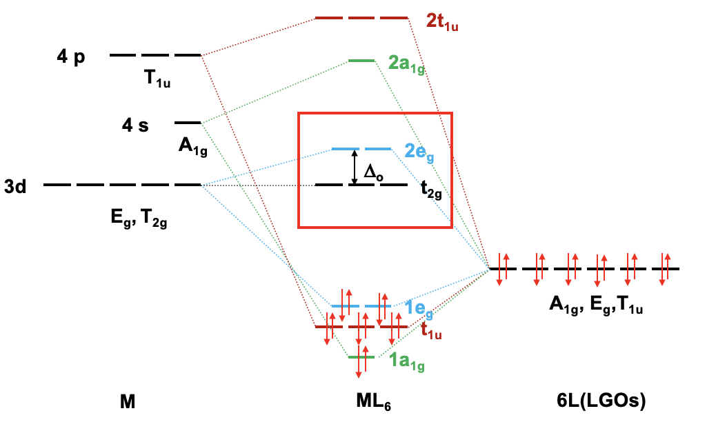
For a 4th row transition metal the sequence of energy is 3d<4s<4p. It makes sense to assume that the ligand group orbitals have about the same energy as the 3d orbitals of the metal, and we can plot them accordingly. Next, we can assign the orbitals their previously determined symmetry types. Then, we can start to combine orbitals of the same symmetry types to form molecular orbitals. We can start for instance with the orbitals having the symmetry type A1. The 4s orbital has that symmetry type. Also one ligand group orbital is of this type. Therefore, we would expect one bonding and one anti-bonding molecular orbital. We can label them 1a1g and 2a1g, respectively, and connect them with the A1g atomic and ligand group orbitals by dotted lines. Next, for example, we can consider the Eg orbitals. There are two metal d orbitals and two ligand group orbitals of that symmetry. We therefore produce two doubly degenerate bonding, and two doubly degenerate anti-bonding molecular orbitals. We can label them 1eg and 2eg respectively. We can further see, that there are the three T1u metal 4p orbitals that we can combine with the ligand T1u orbitals. This gives three triple-degenerated bonding orbitals and three triple-degenerated anti-bonding orbitals with t1u symmetry. Lastly, there are the metal T2g orbitals. There are no ligand group orbitals with the same symmetry, and therefore the T2g orbitals remain non-bonding. We have to write them with unchanged energy into the molecular orbital diagram.
Now we are finished with the construction of molecular orbitals, but still need to fill the electrons into them. We consider the metal-ligand bond a dative bond, with electron pairs being donated by the ligand’s HOMO. Therefore, we consider all ligand group orbitals to be full with electrons. That means that we have overall 6x2=12 electrons to consider. What about the metal electrons? Well, it depends now which metal ion we have. Let us assume here that we have a d0 metal ion with no d electrons. That means that we overall have 12 electrons that we need to fill into the molecular orbitals according to energy. This fills the 1a1g, three t1u, and the two 1eg orbitals. Now let us assume that we would not have a d0 metal ion, but a metal ion with d electrons. There could be up to ten d electrons. Where would they go? They would go into the five orbitals with the next highest energies. Which ones are these? Well, these are the t2g and the 2eg orbitals. The t2g orbitals are the non-bonding metal dxz, dxy, and dyz orbitals, therefore these orbitals are located only at the metal. The 2eg orbitals are anti-bonding molecular orbitals that have been constructed from the dz2 and the dx2-y2 orbitals, and are similar in energy to the dx2-y2 and dz2 orbitals. We can therefore say that the t2g and the 2eg orbitals are the d orbitals under the influence of an octahedral ligand field. Due to the presence of the ligand field the energies of the metal d-orbitals split and the difference in energy is the octahedral ligand field energy \(\Delta\)o. Now we can see that there is an interesting analogy to the crystal field theory. Like the d-orbitals split in energy under an octahedral crystal field into t2g and eg orbitals, the d-orbitals split in energy in an octahedral ligand field into t2g and eg orbitals. Like in crystal field theory the energy of the dz2 and the dx2-y2 is raised. The energy of the other three d-orbitals is unaffected similar, but not exactly the same as the dxy, dyz, and the dxz orbitals in an octahedral crystal field.
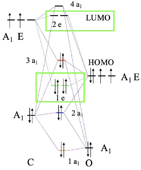
Now we have understood the σ-bonding in an octahedral complex, next let us consider the π-bonding. That means that we have to think about what orbitals of the ligand has the right symmetry for π-bonding with the metal. They should also have an energy similar to the metal orbitals so that significant covalent interaction can occur. We shall stick with our carbonyl ligand, thus we need to look into the molecular orbital diagram of the CO molecule again, and see if there are molecular orbitals suitable for π-bonding (Fig. 7.1.24). The CO molecule has the 1e and the 2e orbitals, that are bonding and anti-bonding π-orbitals, respectively. We can understand this when considering that they are constructed from the 2px and the 2py orbitals that overlap in π-fashion to make the π-bonding in the molecule. Each ligand has two 1e and two 2e orbitals which gives overall four orbitals. These orbitals are energetically similar to the HOMO, thus we can expect that they are energetically close enough to the energy of d-metal orbitals, and can get involved in bonding. We have six ligands meaning that we have 6x12=24 orbitals overall. The twelve 1e orbitals are bonding π-orbitals, and the twelve 2e orbitals are anti-bonding π*-orbitals.
Why are these orbitals suitable for π-bonding with metal d-orbitals? Let us look at their shape, and how they can overlap with a metal d-orbital (7.1.25).
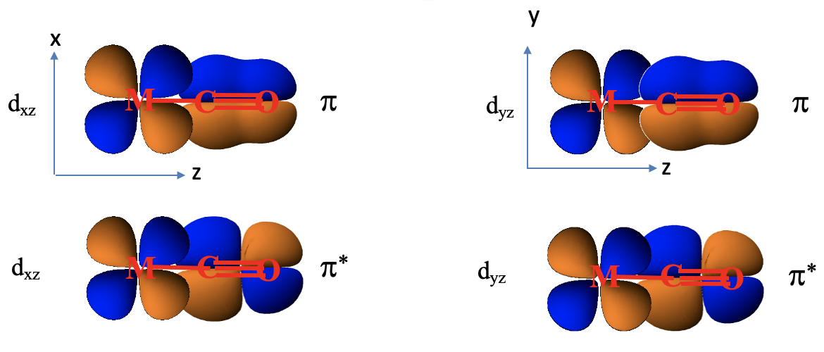
Look for example at a 1e orbital constructed from two 2px orbitals, and how it is oriented relative to the metal-ligand bond axis which we shall define as the z-axis. Next, let us consider a metal dxz orbital orbital. We can see that it is in plane with the 1e orbital, and that the overlap between the dxz and the 1e orbital occurs in π-fashion. Now let us consider the analogous π*-orbital. We can see that it has an additional node, but it can also overlap with a dxz orbital in π-fashion. The ligand does not only have π and π*-orbitals through overlap of two 2px orbitals, but also π and π*-orbitals that result from the overlap of two 2py orbitals. Those orbitals can overlap in π-fashion with a metal dyz orbital. So far, we considered the interactions of a single ligand with the metal only. There are five other ligands, one also approaching from the z-axis, and the other four approaching from the x and y axes. They also have the π and π*-orbitals that interact with the dxz, the dyz, or the dxy orbitals in π-fashion, depending on the direction of approach.
So what do we do with all these orbitals? We group the twelve bonding ones to form a set of ligand group orbitals, and group the twelve anti-bonding ones to form another set of ligand group orbitals. We determine the symmetry types of each set by first determining the reducible representation, and then the irreducible representations using the reduction formula. The result of this process is that the twelve bonding ligand group orbitals have T1g, T2g, T1u, and T2u symmetry. This means that there are three triple-degenerated ones that have T1g symmetry, three other triple-degenerated ones that have T1u, symmetry, three more triple-degenerated ones that have T1u symmetry, and another three triple-degenerated ones that have T2u symmetry. The twelve anti-bonding ligand group orbitals have the same symmetry types. Three have T1g symmetry, three have T2g symmetry, three have T1u symmetry, and another three have T2u symmetry.
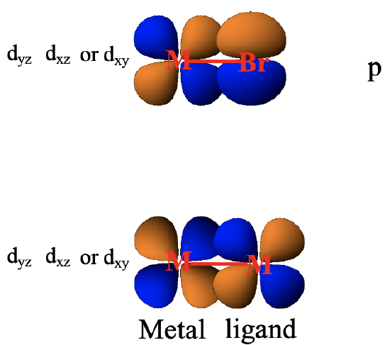
It should be mentioned that there are a number of other orbitals that can make π-interactions when the ligand is not a CO ligand. For example halogenide ligands have p-orbitals that have suitable orientation to overlap with metal d-orbitals in π-fashion (Fig. 7.1.26). When there are complexes with metal-metal bonds then there is also the possibility of metal d-orbitals to overlap with other metal d-orbitals in π-fashion.
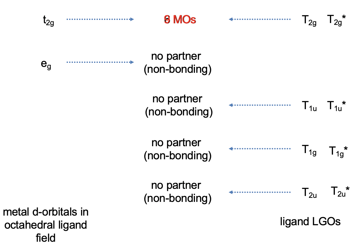
Now that we have determined the symmetry types of the ligand group orbitals available for π-bonding, we need to select those ligand group orbitals that have suitable symmetry to form molecular orbitals with metal d-orbitals in the octahedral ligand field. These are the 2eg and the t2g MOs that resulted from the σ-interactions. For simplicity sake we will call the 2eg molecular orbitals just the metal eg orbitals. The t2g MOs are identical to the metal T2g atomic orbitals because the metal T2g atomic orbitals remain exactly non-bonding with respect to σ-interactions. The ligand group orbitals have T1g, T2g, T1u, and T2u symmetry respectively. That means that we can combine the t2g metal orbitals and the T2g ligand group orbitals to form molecular orbitals. The metal eg orbitals and the ligand T1g, T1u, and T2u orbitals remain non-bonding because they do not find a partner (Fig. 7.1.27). The three bonding T2g LGOs will form six MOs of the same symmetry type with the three metal t2g orbitals. In addition, we need to consider that there are also three anti-bonding T2g* LGOs that were formed from the anti-bonding π-orbitals. They can also interact with the metal t2g d-orbitals. Because the number of MOs of a given symmetry type is always the sum of the atomic orbitals + the LGOs of that symmetry type this adds three MOs to the six MOs giving overall nine t2g MOs. There are also the T1u*, the T1g*, and the T2u* orbitals. They just remain non-bonding because they do not find a partner.
We can now think of two extreme cases for the combination of the metal t2g with the ligand T2g and T2g* orbitals. In the first case the T2g LGOs are much closer in energy to the metal t2g orbitals, and the T2g* LGOs are energetically much higher than the metal t2g orbitals. In this case we can neglect the covalent interactions between the T2g* orbitals and the metal t2g orbitals, and the T2g* orbitals remain effectively non-bonding. We would consider only the interactions between the T2g LGOs and the metal t2g orbitals to form three bonding and three anti-bonding MOs of t2g symmetry (Fig. 7.1.28). Now we need to consider the electrons. The bonding T2g LGOs are full, and therefore there are overall six electrons to consider. These six electrons would go into the three bonding t2g MOs. Now can also have up to ten metal d electrons. Six of them can be accommodated by the t2g metal orbitals, the other four would be in the eg orbitals. Upon the formation of the π-bond, the t2g metal electrons will be in the anti-bonding t2g orbitals. The eg electrons will simply remain non-bonding. We can see that the π-interactions lower the energy of the ligand electrons, but increase the energy of the metal electrons. If we get a net stabilization of electron energies will depend on how many d electrons we have. As long as there are less than six d electrons we will see a stabilization, if there are more there will be an overall destabilization. We can also ask what impact the π-bonding has on the magnitude of the Δo. We can see that the π-bonding decreases the Δo. It is larger before the bonding compared to after the π-bonding.
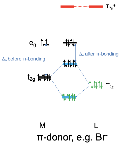
We call a ligand that has T2g orbitals of similar energy to the metal t2g orbitals, and T2g* orbitals of much higher energy compared to the metal t2g orbitals a π-donating ligand, or a π-donor (Fig. 7.1.28). This is because before the π-bonding the ligand electrons are localized exclusively at the ligand, and after the π-bonding they are in the bonding t2g MOs which are shared between the metal and the ligand. Thus, a partial electron transfer has occurred from the ligand to the metal. An example for π-donating ligands are halogenide ligands such as a bromo ligand.
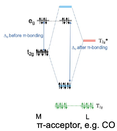
Now let us consider the opposite case in which the anti-bonding T2g* ligand orbitals are energetically close to the metal t2g orbitals and the bonding T2g ligand orbitals are energetically too low in order to significantly interact with the metal t2g orbitals. This means that the T2g-orbitals remain practically non-bonding. The T2g* ligand group orbitals and the metal t2g orbitals form three triply degenerated bonding molecular orbitals and three triply degenerated anti-bonding molecular orbitals. Because the T2g* ligand group orbitals are empty, no ligand electrons are filled into the new molecular orbitals. This means that up to six metal d electrons can be filled into the bonding molecular orbitals of t2g symmetry. Any remaining d electrons in the eg orbitals just remain in the eg orbitals and do not change in energy. We can see that in contrast to the previous case, we can lower the energy of the metal d electrons through π-interactions. Because the bonding t2g electrons are shared between the metal and the ligand, electron density has been transferred from the metal to the ligand. Therefore, a ligand that primarily utilizes its anti-bonding T2g*-orbitals for π-bonding is called a π-acceptor ligand, it accepts d-electron density from the metal. An example for a π-acceptor ligand is the carbonyl ligand (Fig. 7.1.29). It is also important to understand the influence of a π-acceptor ligand on the size of Δo. Because the anti-bonding t2g MO is higher in energy than the non-bonding eg orbitals, the Δo is now defined by the energy difference between the bonding t2g MOs and the eg orbitals (Fig. 7.1.29). We can see that Δo is increased when π-acceptor interactions are taken into account.
We have now discussed the two extreme cases, however there are many ligands that are actually in between these two extremes, and there is a continuous spectrum from strongly π-donating, to weakly π-donating, to weakly π-accepting, to strongly π-accepting ligands. It is also possible that π-donor and π-acceptor effects cancel out. This is the case when the the T2g and T2g*-ligand group orbitals are energetically about equidistant to the metal t2g orbitals. Some ligands also do not have orbitals suitable for π-bonding at all, and there are neither π-donating nor π-accepting effects.
The effect of π-bonding on Δo can nicely explain the spectrochemical series. Because π-accepting ligands increase Δo, these complexes absorb light of shorter wavelength and of higher energy. π-donating ligands decrease Δo and and thus lead to the absorption of light having longer wavelengths. We see here that the ligand field theory is more powerful than the crystal field theory. The latter was not able to explain why different ligands produce different Δo values.
Ligand field theory is also able to nicely explain the magnetism of coordination compounds, and high and low spin complexes in particular. It is also able to explain why certain ligands tend to produce low spin complexes, while others tend to form high spin complexes. According to ligand field theory π-acceptors tend to make low spin complexes, and π-donors tend to make high-spin complexes. This is in accordance with experimental observation.
Octahedral Complexes and The 18 Electron Rule
Figure 7.1.30 Qualitative MO diagram of the octahedral hexacarbonyl chromium complex under consideration of \(\pi\)-bonding.
Another great feature of ligand field theory is that it can explain the 18 electron rule, and exceptions from the 18 electron rule. For example, the octahedral hexacarbonyl chromium complex is an 18 electron complex. Let is construct a qualitative molecular orbital diagram and see if the MO diagram supports the stability of the complex. The MO diagram considering only the σ-interactions is shown in Fig. 7.1.30. We can see that all the twlelve ligand electrons are in the bonding molecular orbitals 1a1, 1tu, and 1eg. In addition the chromium has six valence electrons. These electrons remain non-bonding when considering σ-interactions only. However, this changes, when we consider π-interactions. The CO ligand is a strong π-acceptor ligand, therefore we consider only its T2g* π-ligand group orbitals for bonding. They must be located energetically above the LGOs for σ-bonding. The interaction of the metal t2g orbitals creates three bonding t2g MOs and the three anti-bonding ones. Because we can fill metal d electrons into the bonding MOs the status of the d-electrons has changed from non-bonding to bonding. We can see now that all 18 electrons are in bonding MOs, and that no electron is in-non-bonding or anti-bonding MOs. When all electrons are in bonding MOs then this is the ideal situation for complex stability. This is explains why the 18 electron complex is stable. If we analyzed the MO diagrams of many other stable 18 electron complexes then we would also mostly find that all bonding MOs are filled, and all other MOs are empty. This explains the 18 electron rule.
Figure 7.1.31 The qualitative molecular orbital diagram of WCl6 under consideration of \(\pi\)-bonding.
Next, let us construct a qualitative molecular orbital diagram of WCl6. This is not an 18 electron complex, it has only twelve electrons coming from the six chloro ligands. W is in the oxidation state +6 and is a d0 species contributing no electons. Can ligand field theory explain this exception from the 18 electron rule? Let us again start with the MO diagram considering σ-bonding only. The twelve ligand electrons go into the bonding 1a1g, 1tu, and 1eg orbitals. The non-bonding t2g and the anti-bonding 2eg orbitals remain empty due to the absence of metal d electrons. We can see that all bonding molecular orbitals are full and all others are empty, explaining the stability of the molecule, and thus the exception from the 18 electron rule. Now let us consider π-bonding in addition. A chloro ligand is a typical π-donor which uses its 3p electrons that are suitably oriented for π-bonding. Therefore, we only consider the T1g ligand group orbitals for bonding here. These orbitals are full with electrons because a chloride anion has a full 3p subshell. The interaction of the T2g LGOs with the metal t2g orbitals creates a bonding t2g MO and an anti-bonding t2g MO. We can see that the ligand π-electrons now have a lower energy than without the π-interactions of the metal. Therefore, the π-bonding has further stabilized the complex. In a way, we can now even say that we have an 18 electron complex because when we add th 6 π electrons to the 12 σ electrons we get 18 bonding electrons overall. These additional 6 electrons are not accounted for in electron-counting because electron-counting treats the W-Cl bond as a single bond and only considers the σ-interactions between W and Cl.
Tetrahedral complex of a 4th period Transition Metal
Next, let us consider a tetrahedral complex and see if ligand field theory can explain it well. The point group for a tetrahedron is Td, and we will need the character table of this point group (Fig. 7.1.32)
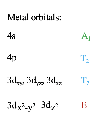
We choose the coordinate system like in the crystal field theory. We inscribe the tetrahedron into a cube by occupying every other vertice of the cube with a ligand (Fig. 7.1.34). Then, we let the axes run perpendicular to the faces of the cube. Next, we need to think about the symmetry types of the metal frontier orbitals. For a fourth period transition metal these are the 3d, the 4s, and the 4p orbitals. Looking into the character table of the point group Td gives us their symmetry types (Fig. 7.1.32 and Fig. 7.1.33). The 4s orbital has the totally symmetric symmetry type A1, We find the letters x,y, and z in parentheses in the irreducible representation of the type T2, and this means that the 4p orbitals are triply degenerated and have the symmetry type T2. The 3dxy, the 3dyz, and the 3dxz orbitals are found in the same irreducible representation, are also triple-degenerated, and have T2 symmetry. The 3dx2-y2 and the 3dz2 orbitals have the symmetry type E according to the character table for Td.
Now we need to think about the ligands. Because we need to consider σ-bonding first, we have to find the HOMO of the ligand suitable for σ-bonding. We can choose again a carbonyl ligand as an example ligand, and in this case the HOMOs of the CO ligands would be used for σ-bonding. This is actually not immediately obvious. If we chose the coordinate system of the metal and ligands to be same same, then then the CO bond axis, which we previously defined as the z-axis, would not point toward the metal, and no σ-overlap with a metal orbital would be possible. Therefore, we must give each ligand a different coordinate system with the z-axes pointing toward the metal (Fig. 7.1.34). Only then, the CO molecule would point toward the metal, and would be oriented to make σ-bonding with the metal. Generally, when constructing MOs, the ligands should always be oriented to that bonding is maximized. This is usually the case when orbital overlap for σ-bonding is maximized.
Figure 7.1.34 A tetrahedral complex inscribed in a cube with CO ligands each having its own coordinate system.
Because we have four ligands we will have four ligand HOMOs that we would group to form four ligand group orbitals. Which symmetry types do they have? In order to obtain the symmetry types we would need to determine the reducible representation first, and then the irreducible representations this reducible representation is composed of. We won’t do this explicitly here and not go through the entire mathematical process, and only consider the results.
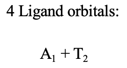
The result is that one ligand group orbital has the symmetry type A1 and the other three have the symmetry type T2 (Fig. 7.1.35).
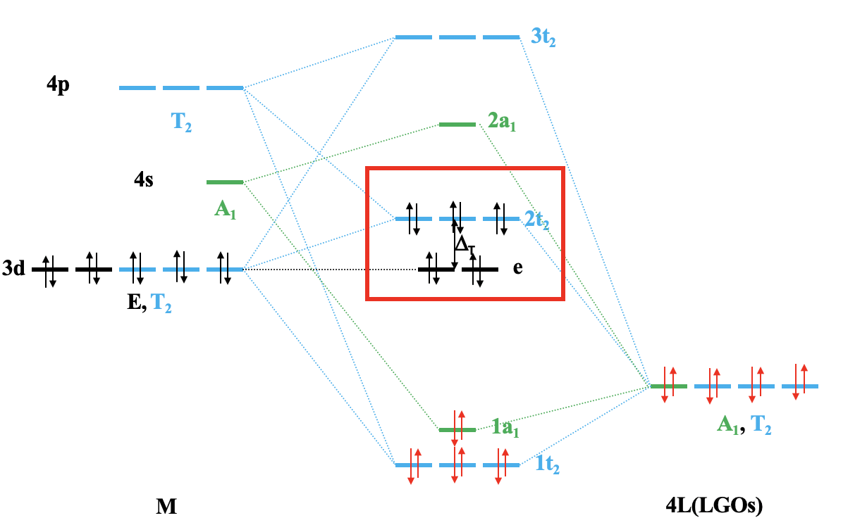
We can now construct the molecular orbital diagram for σ-bonding (Fig. 7.1.36). First, we can plot the metal frontier orbitals according to the energy on the left side of the diagram, and label the orbitals according to their symmetry types. On the right side we plot the four ligand group orbitals, and label them according to their symmetry type. Their energy should be approximately that of the metal d-orbitals. Now we can construct molecular orbitals by combining atomic and ligand group orbitals of the same symmetry type. The 4s orbital and one LGO have A1 symmetry, and therefore we can combine them to form a bonding 1a1 and an anti-bonding 2a1 orbital. Next, let us direct our attention to the t2 symmetry type. The 4p and three metal d orbitals have that symmetry type, and so have three LGOs. That is overall nine orbitals, so we must get nine MOs with t2 symmetry. Because of triple-degeneracy, there must be three sets of triple-degenerate MOs. We can estimate that one set will be bonding, one will be approximately non-bonding, and one will be anti-bonding. We can label them 1t2, 2t2, and 3t2 respectively. The 2t2 is actually somewhat anti-bonding in nature. Now only the metal e-orbitals are left. They do not find a partner and remain non-bonding.
We still need to fill the electrons into the MOs. The four ligand HOMOs are considered full, which gives 4×2=8 electrons. The electrons occupy the bonding 1t2 and the 1a1 orbitals explaining the four dative metal-ligand bonds. All metal d electrons, which could be up to ten, would need to go into the e and/or the t2-orbitals. The e-orbitals are the non-bonding dz2 and dx2-y2 orbitals, and the 2t2 orbitals are only weakly anti-bonding and have strong d-metal orbital character because they are have been constructed from the dxy, the dyz, and the dxz orbitals, and are fairly similar in energy to those orbitals. We can therefore say that the the e and the 2t2 orbitals are the metal t2 and eg orbitals in a tetrahedral ligand field. The energy difference between the e and the 2t2 orbitals is the tetrahedral ligand field energy ΔT. You see here again the relationship between ligand and crystal field theory. You can also see that ligand field theory can explain why crystal field theory works as a bonding theory even though it is not an actually bonding theory.
π-bonding in a tetrahedral complex
What is the π-bonding in a tetrahedral complex?
First, we need to decide if there are ligand orbitals that are suitably oriented to overlap with metal orbitals in π-fashion. We can see that no ligand orbital is overlapping with a metal d-orbital exactly in π-fashion, however, the e π and 2e π*-orbitals of the ligands still overlap so that at bonding interaction is created, and this orbital overall occurs similarly to π-overlap. Therefore, we can still approximate the bonding interactions as π-bonding. We need to consider though that because of smaller orbital overlap, the π-bonding in tetrahedral complexes is weaker than in octahedral complexes. How many ligand orbitals will we need to consider? Assuming that we will stick with CO as the ligand, there will be four per ligand, and thus there will be 4×4=16 overall. Of these, there will be eight bonding e π-orbitals and eight anti-bonding e π*-orbitals. We group the bonding ones to form a set of eight ligand group orbitals, and group the anti-bonding ones to form another set of eight anti-bonding ligand group orbitals. What will be their symmetry types? We can determine the reducible representations and irreducible representations to find this out. We are not going through the exact process here, but only look at the results. The result is that each set of ligand group orbitals has the two E-type orbitals, three T1-type, and three T2-type ligand group orbitals.
4_with_pi-bonding.gif?revision=1)
Figure 7.1.38 MO diagram of a tetrahedral complex of a 4th period transition metal (pi-bonding with pi-acceptor)
Since we now know the symmetry of the ligand group orbitals we can combine them with same-symmetry metal d-orbitals in the tetrahedral ligand field to form π-molecular orbitals. Let us do this for the example of nickel tetracarbonyl, a tetrahedral complex of Ni in the oxidation state 0 and four carbonyl ligand. We can use the MO diagram for σ-bonding which we constructed previously as a starting point, and modify it so that it accounts for π-bonding (Fig. 7.1.38).
First, we need to add the new ligand group orbitals to the MO diagram. We only need to consider the E and T2 LGOs and not the T1 LGOs because no metal orbital has t1 symmetry. Next, we need to take into account that the CO ligand is a strong π-acceptor ligand. This means that we only need to consider the LGOs formed from the anti-bonding π*-orbitals. We must draw these orbitals above the LGOs for σ-bonding into the MO diagram because the LGOs for σ-bonding have been formed from the CO HOMOs while the anti-bonding LGOs for π-bonding have been formed from the CO LUMOs. We can now combine the π-LGOs and metal d-orbitals of the same symmetry to form π-MOs. We see that we can combine the e-type LGOs with the non-bonding e-type metal dz2 and dx2-y2 orbitals to form a pair of bonding MOs of e-symmetry, and an anti-bonding pair of e-symmetry, which we can label 1e and 2e, respectively. Now what is the effect on the T2-type π-LGOs? We first need to realize that we have already three sets of triple-degenerated t2-MOs generated through σ-interactions. The interaction of the T2-LGOs with the σ-t2-MOs must create another set of triply-degenerated orbitals so that the overall number of orbitals with t2-symmetry remains the same. The interaction will occur mostly between the 2t2 MO and the T2-LGOs because the 2t2 MOs have the most similar energy to the T2-LGOs. This leads to the lowering of the energy of the 2t2 MOs, so that these formerly weakly anti-bonding orbitals become weakly bonding. The additionally created t2-orbitals are weakly anti-bonding. We can label them 3t2. The former anti-bonding 3t2 –orbital will be re-labeled 4t2. We can double-check that we have constructed the t2-MOs correctly by verifying that the number of T2-LGOs, and that includes σ and π, plus the number of metal T2 orbitals equals the number of t2 molecular orbitals. We see that the number of metal T2 orbitals + the number of T2 LGOs is 6+6=12. The number of t2 MOs is 4×3 which is also 12.
Finally, we still need to fill the electrons. As previously mentioned, the π-LGOs as empty and therefore the ligand does not contributed any electrons to the π-bonding. The Ni is in the oxidation state 0 and thus contributes 10 electrons because Ni is in the 10th group of the periodic table. Because a neutral Ni atom has the electron configuration 3d84s2 we can draw eight electrons in to the 3d orbitals and two electrons into the 4s orbitals. The 1t1 and the 1a1 MOs are already full with ligand electrons due to σ-bonding. Thus, the metal electrons must go into the 2e and the 2t2 MOs. Both the e-orbitals and the 2t2-orbitals are bonding, and thus we can say that the metal d-electrons have been stabilized due to the π-acceptor nature of the ligand. We see here an analogy to the octahedral ligand field. Like in the octahedral ligand field π-acceptor ligands tend to lower the energy of the metal d-electrons. We can also ask: What is the effect of a π-acceptor ligand on ΔT? The answer is: Like Δo gets larger in the octahedral ligand field, ΔT gets larger in a tetrahedral ligand field. However, the increase is much smaller compared to the octahedral field. Why? this is because in the octahedral ligand field, the energy of the eg orbitals is not affected through the π-acceptor interactions, and only the t2g orbitals are lowered in energy. In the case of the tetrahedral ligand field both the energy of the e and the t2 orbitals get lowered, and the energy of the e-orbitals gets only slightly more lowered than the energy of the t2 –orbitals. Therefore, the ΔT only slightly increases. This fact can also serve as an additional explanation why tetrahedral complexes never make low-spin complexes, even with strong π-accepting ligands. The effect of the ligand on ΔT is simply still too small because both the energy of the e and the t2 orbitals have been lowered.
Finally, let us discuss the results in the context of the 18 electron rule. We can see that the number of electrons involved in σ-bonding are in bonding molecular orbitals. Thus, it is justified to say that the ligand field theory is able to explain the 18 electrons rule.
Figure 7.1.39 MO diagram of a tetrahedral complex of a 4th period transition metal (\(\pi\)-bonding with \(\pi\)-donor)
Now let us think about how a π-donating ligand influences the magnitude of ΔT. In this case we only need to consider the bonding E and T2 ligand orbitals if the ligand has π-bonds. Those orbitals will be energetically below the LGOs for σ-bonding. If the ligand is a simple ion like chloride, then we would consider LGOs from the filled p-orbitals that that have suitable symmetry for π-overlap. Those LGOs would have the essentially the same energy as the σ-LGOs. Let us construct a qualitative MO diagram of TiCl4 which has chloro ligands which are typical π-donating ligands. When constructing the MO diagram for π-bonding we can again start with the MO-diagram for σ-bonding, and then modify this diagram. We can first plot the filled π-T2 and Eg LGOs with similar energy as the σ-LGOs on the right side of the diagram. The E ligand group orbitals will now interact with the e-metal orbitals. That interaction leads to a pair of bonding MOs of e-symmetry, and a pair of anti-bonding MOs of e-symmetry. This means that effectively, the formerly non-bonding e-metal orbitals become anti-bonding MOs, and move up in energy. The bonding e-type MO is created in addition and must have lower energy than the E-type π-LGOs. The interaction of the T2-LGOs with the metal t2-orbitals creates an additional set of bonding t2-orbitals. The 2t2 orbitals move up in energy, and become more anti-bonding, as a consequence of that. We can just renumber the t2 and the e MOs. Now we still need to fill the electrons into the MOs. The π-LGOs have overall eight electrons. These electrons will go into the newly formed bonding 1e and 1t2 molecular orbitals. We see that this leads to a stabilization of these electrons. This is an analogy to the octahedral ligand field. When we have a π-donor ligand, then that the π-ligand electrons. What about the metal electrons. In TiCl4 the Ti is in the oxidation state +4, therefore it is formally d0, and it does not have any electrons. This explains the stability of the TiCl4 as complex that does not obey the 18 electron rule. It has only 8 electrons, but the bonding situation is nonetheless ideal. All bonding MOs are full, and all others are empty. If the Ti had d electrons they would need to go into the 2e and the 3t2 orbitals which are both anti-bonding. This would destabilize the complex. In general π-donating ligands increase the energy of metal d-electrons, and this is another analogy to the octahedral ligand field. Now to the question, what is the effect of a π-donating ligand on ΔT? Both the metal e and t2 frontier orbitals have increased in energy but the e-orbitals more so than the t2 orbitals. That means that the ΔT has overall decreased. This is a further analogy to the octahedral ligand field. π-donating ligands lead to a smaller ΔT.
Overall the ligand field theory can again provide an explanation for the spectrochemical series. π-donors lead to smaller ΔT ligands, and thus the complex absorbs light of larger wavelengths, π-acceptors lead to larger ΔT and those complexes absorb light of smaller wavelengths.
Square Planar Complex of a 4th Period Transition Metal
As a last example we will discuss now the molecular orbital diagram of a square planar complex. This will be the most complicated MO diagram we will discuss. The greater complexity stems from the lower symmetry in a square planar complex. It belongs to the point group D4h whereas tetrahedral and octahedral complexes belong the high symmetry point groups Td and Oh.
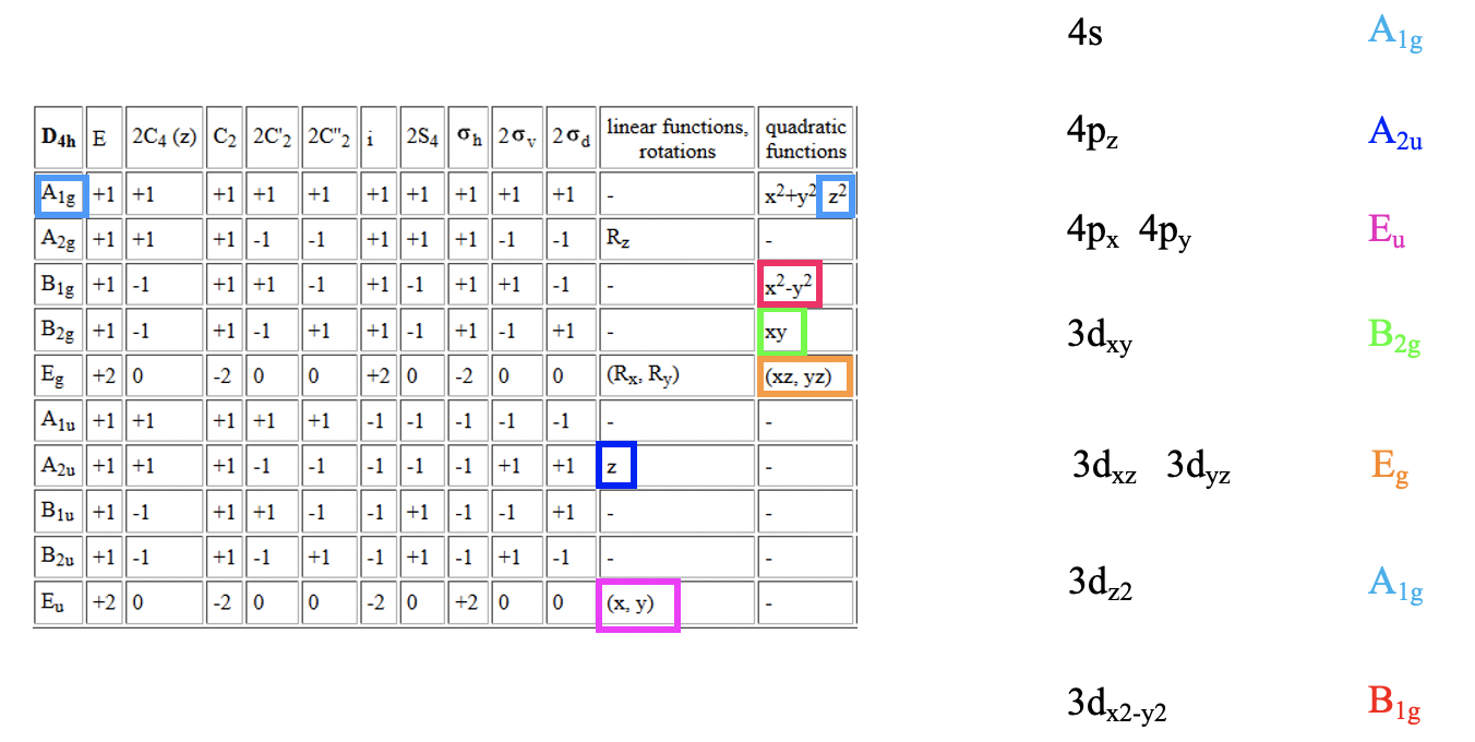
The lower symmetry leads to a reduction in the degeneracy of the molecular orbitals. This creates more energy levels and hence a more complicated molecular orbital diagram. Let us think next about the definition of the axes. I would be sensible to define the xy plane as the plane of the molecule with the x and the y-coordinates going through the bonds. The z-axis would stand perpendicular to the plane of the molecule. What are the symmetry types of the metal frontier orbitals. Assuming a 4th period transition metal the 3d, the 4s, and the 4p orbitals would be the frontier orbitals. Looking into the character table of the point group D4h (Fig. 7.1.10) shows that the symmetry of the 4s orbital is A1g, the symmetry of the 4p orbitals is A2u for the 4pz orbital and eu for the 4px and the 4py orbitals. The d orbitals have the symmetry types A1g, B1g, B2g, and Eg for the 3dz2, dx2-y2, 3dxy, and 3dxz/3dyz, respectively.
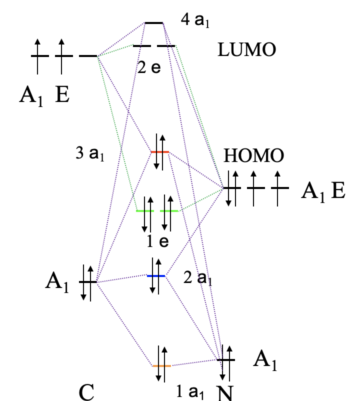
Next, we to determine the ligand HOMOs suitable for σ-bonding. There are no square planar carbonyl complexes, therefore we will not choose the carbonyl ligand as a example ligand here. Instead we will use the related cyano ligand. The cyano ligand is isoelectronic with the carbonyl ligand. Formally, the O-atom in CO is replaced by N. Because N has one electron less than O, we must add one electron, giving the cyano ligand a 1- negative charge. Like in CO, the cyano ligand has a triple bond between C and N, and there is an electron lone pair at C, and one at N. The MO diagram is similar to that of CO, just the energy difference between C and N orbitals is somewhat smaller than that of the energy difference between C an O orbitals (Fig. 7.1.41). The number, symmetry, and energy order of the MOs of CN- and CO is the same. Therefore, the CN- has the same HOMOs suitable for σ-bonding, and we can select it for the construction of σ-MOs. Each ligand has one HOMO, therefore we have overall four HOMOs.
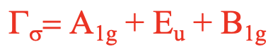
We can group them to form LGOs and determine the symmetry types of the LGOs. The result is that there is on ligand group orbital with A1g symmetry, there are two with Eu symmetry, and there is one with B1g symmetry (Fig. 7.1.42).
Square Planar Complex: σ-bonding
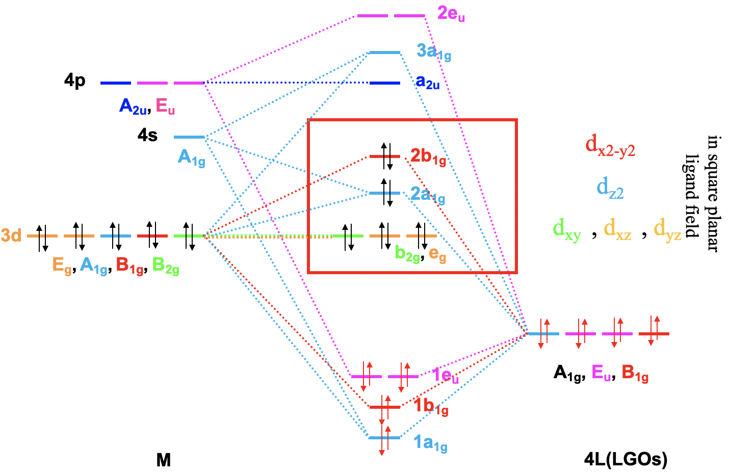
We have now the all information necessary to construct a qualitative molecular orbital diagram for σ-bonding (Fig. 7.1.43). As usual we first plot the metal frontier orbitals on the left and the ligand group orbitals on the right side of the MO diagram, and label the symmetry types. Then, we need to combine metal frontier and ligand group orbitals of the same symmetry type to form molecular orbitals. We can for instance begin with the symmetry type A1g. The 4s orbital and the 3dz2 orbitals have this symmetry type, and so has one ligand group orbital. We will therefore get three molecular orbitals of that symmetry type, a bonding one, an approximately non-bonding one, and an anti-bonding molecular orbital. We plot them according to their expected energy into the MO diagram, and label the MOs 1a1g, 2a1g, and 3a1g, respectively. Next, we can look at the B1g orbitals. The 3dx2-y2 orbital and one LGO of that symmetry type, and thus we can form a bonding and an anti-bonding MO from this combination. We can further see that we can combine the 4px and the 4py orbitals that have Eu symmetry with the remaining two LGOs of the same symmetry. This gives two double-degenerated bonding MOs of eu symmetry, and two anti-bonding bonding ones of the same symmetry. Are there any orbitals with other symmetry types left? Yes, there are the metal dxy, dxz, and dyz orbitals that have B2g, and Eg symmetry, respectively, In addition, there is the pz orbital that has a2u symmetry. We can see that these metal orbitals do not find a partner. There is no LGO of these symmetry types. We therefore have to draw these orbitals as non-bonding orbitals into the MO diagram.
Now it is the time to fill the electrons into the molecular orbitals. The LGOs are occupied with electrons because they have been formed from the HOMOs of the ligand. Because we have four LGOs we have eight electrons to consider. These electron will therefore fill the 1a1, the 1b1g, and the 1eu molecular orbitals. These orbitals are all bonding molecular orbitals. Thus, ligand field theory is able to explain the four bonds and the square planar shape of the molecule. Where would the metal d-electrons go? We could have up to ten d-electrons depending on the metal ion, and these ten electrons would go into the five MOs of the next higher energy. These are the non-bonding b2g and eg orbitals, the approximately-non-bonding 2a1g orbital, and the anti-bonding 2b1g orbital. We can consider these orbitals as the metal-d-orbitals in a square planar ligand field. The b2g orbitals is the dz2 orbital in the square planar ligand field, the eg orbitals are dxz and dyz in a square planar ligand field, the 2a1g orbital is the dz2 orbital in a square planar ligand field and the 2b1g orbital is the dx2-y2 orbital in a square planar ligand field. We can see that these results are similar yet not completely analogous to those we obtained in the crystal field theory. Remember, that in the crystal field theory the dx2-y2 orbital had also had the highest energy. However, the dz2 was lower in energy than the dxy, and the dxy was not degenerate with the dxz and the dyz orbitals. The difference it due to the fact that in ligand field theory the dxy orbital is considered non-bonding, not interacting with the ligands at all, whereas in crystal field theory a strong electrostatic repulsion between the dxy and the ligands is assumed because the dxy orbital is in the plane of the molecule.
Square Planar Complex π-bonding
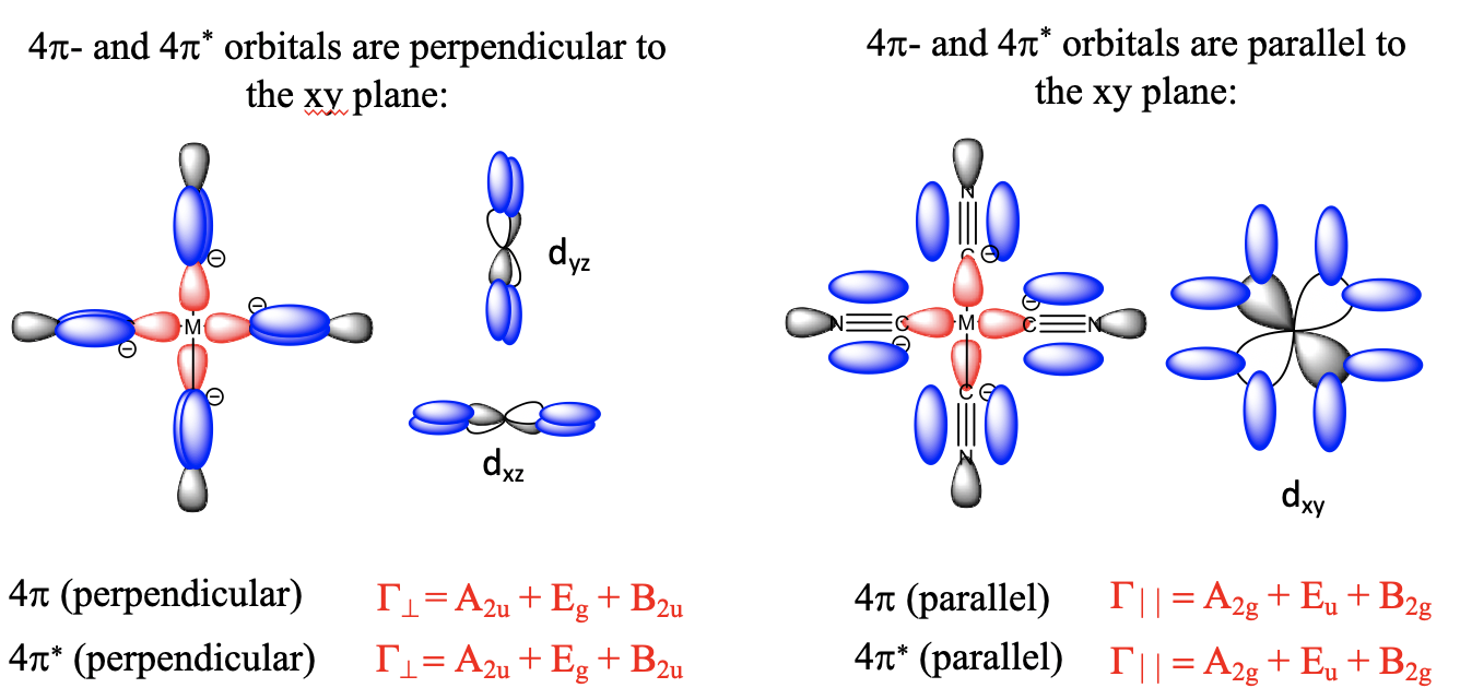
Now let us look at the π-bonding of a square planar transition metal complex (Fig. 7.1.44). If we assume a CN- ligand, then the orbitals that have suitable symmetry to overlap with the metal frontier orbitals in π-fashion are the 1e and 2e π and π* orbitals from the MO diagram of CO. There are two π and two π* orbitals per ligand. Because we have four ligands there are overall eight π and eight π* orbitals. Now we need to consider that four of the π-orbitals are in the xy plane, while the other four are above and below the xy plane. We call the former the parallel orbitals, and the latter the perpendicular orbitals, because they are oriented parallel and perpendicular to the xy plane, respectively. We must distinguish them because they have a different symmetry and overlap differently with the metal d-orbitals. This is illustrated for the bonding π-orbitals in Fig. 7.1.44. The anti-bonding ones behave analogously. Therefore we group the orbitals to form four sets of ligand group orbitals π⊥ , π||, π*⊥ , and π*||. Our next task is to determine the symmetry types of these orbitals. We again omit the exact process, but only look at the results. Both the π⊥ and the π*⊥ orbitals have one A2u, two Eg and one B2u ligand group orbitals. The π|| and π*|| orbitals have one A2g, two Eu, and one B2g ligand group orbitals.
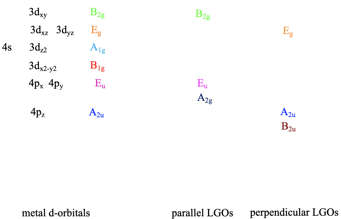
We now need to add the π-molecular orbitals to the molecular orbital diagram that we had constructed previously to account for σ-bonding. First, we need to consider which π-LGOs have the right symmetry to produce π-MOs with metal d-orbitals (Fig. 7.1.45). We can see that among the parallel LGOs the A1g and the B1g orbitals find partners, but not the Eu orbitals, For the perpendicular LGOs the Eg orbitals find partners, but not the A2u and the B2u orbitals. We therefore only need to consider the A1g, the B1g and the Eg LGOs. To make matters more complicated, to get a realistic MO diagram for a square planar complex with cyano ligands it is necessary to consider the interactions of the 4s and the 4p orbitals with the π-LGOs as well. The symmetry of the 4s was A1g and the symmetry of the 4p orbitals was A2u and Eu, respectively. The 4s still does not find a partner, but the 4p orbitals do.
MO Diagram of a Square Planar Complex With a Cyano Ligand
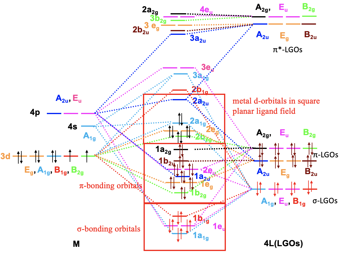
Let us now construct the MO diagram of a square planar complex with a cyano ligand considering both σ and π-bonding for the example of the Ni(CN)42- complex anion. Because of the complexity of the diagram we will not modify the MO diagram for σ-bonding, like we did previously, but construct the complete MO diagram from scratch (Fig. 7.1.46). Like previously we can plot the metal 3d, 4s, and 4p orbitals on the left side of the diagram. On the right side of the diagram are now the LGOs for σ as well as π-bonding. For the Ni(CN)42- complex the σ-LGOs are energetically somewhat below the metal d-orbitals, the bonding π-LGOs have about the same energy as the metal d-orbitals, and the anti-bonding π*-LGOs have an energy significantly higher than the 4p orbitals. We can again construct MOs symmetry type by symmetry type until the MO diagram is complete. We can start with the symmetry type A1g. We see there is only one σ-LGO that interacts with the 4s and the 3dz2 which also have A1g symmetry. That leads to a bonding, an approximately non-bonding, and anti-bonding a1g MO which we can label 1a1g, 2a1g, and 3a1g, respectively. Next, we can for instance look at the B2g orbitals. There is one d-orbital that has that symmetry, as well as two LGOs. The interaction is almost only with the bonding B2g LGO because the energies are similar. This leads to a bonding and an anti-bonding π-MO with B2g symmetry. The anti-bonding LGO is too high in energy and it does not significantly interact. Therefore we can draw it with the same energy into the MO-diagram. Now let us go to the B1g orbitals. There is a metal d-orbital with B1g symmetry, and a σ-LGO with B1g symmetry. This produces a bonding and anti-bonding MO with B1g symmetry. Now let us go to the Eg orbitals. There are two Eg metal d-orbitals, two Eg π-LGOs and two Eg π*-LGOs. Again, the π*-LGOs are too far off in energy, so that the bonding interaction is mostly between metal orbital the π-LGOs. This leads to a pair of bonding MOs and a pair of anti-bonding MOs. The π*-LGOs can be drawn with unchanged energy into the MO-diagram. The 4p orbitals of the metal have symmetry types, we have not considered yet: A2u and Eu. Let us begin with the Eu orbitals. There are two σ-Eu LGOs, two π-Eu-LGOs and two π*-Eu LGOs. Overall we have four pairs of EU-orbitals, and we would therefore expect four pairs of eu-MOs. We can make the approximation that there will be a bonding one, a weakly bonding one, a weakly anti-bonding one, and a strongly anti-bonding one. We can label them 1eu, 2eu, 3eu, and 4eu, respectively. The 4eu has almost only contributions from the anti-bonding π*-EU LGOs due to energy arguments, therefore it is only connected to these via a dotted line, and not to the other Eu orbitals. Now to the A2u orbitals: There is a π and a π*-orbital of A2u symmetry that can be combined with the 4p A2u orbitals. This leads to three A2u MOs overall, one bonding, one approximately non-bonding, and one anti-bonding one. Now we have used all metal d-orbitals. We notice that there are still some LGOs that we have not used. These are the π and π* A2g and the B2u LGOs. They remain non-bonding can be drawn accordingly in the MO diagram.
We now need to fill the electrons into the MO-diagram. Firstly, there are the σ-electrons to consider. There are overall eight electrons stemming from the four occupied σ-LGOs. We can fill these eight electrons into the four MOs with the lowest energy. These are the 1a1, the 1eu and the 1b1. These are all bonding MOs explaining the four σ-bonds within the complex. We can call these four orbitals the σ-bonding orbitals. Next we need to consider the electrons in the π-LGOs. There are overall eight of these orbitals containing 16 electrons. We must fill these electrons into the eight MOs of the next-higher energies. These are the 1b2g, the 1eg, the 1a2u, the 2eu , the 1b2u, and the 1a2g orbitals. We see that these orbitals are either bonding or non-bonding, and thus overall the ligand π-electrons get stabilized due to the π-interactions with the ligand. We can call these orbitals the π-bonding molecular orbitals. Finally we need to look at the metal d-electrons. We assume Ni as the metal with Ni in the oxidation state +2 and d8 electron configuration. We need to fill these eight electrons into the four next higher-energy MOs. This fills the 2b2g, the 2eg, and the 2a1g, orbitals which are either non-bonding or anti-bonding. This means that the metal electrons are overall destabilized. This behavior is consistent with the cyano-ligand acting as a π-donating ligand. We understand from this why square planar complexes prefer 16 over 18 electrons and disobey the 18 electron rule. If we had two more electrons then these would need to go into the energetically much higher 2a2u orbitals. The energy gap between the 2a2u and the 2a1g orbital is significantly higher than that between the 1a1g, the 2b2g, and the 2eg orbitals. Overall we can call the 2au, the 2a1g, the 2eg, and the 2bg orbitals the metal d-orbitals in a square planar ligand field. In a square planar ligand field we have three ∆s. ∆3 is the energy difference between the 2b2g and the 2eg orbitals, ∆2 is the energy difference between the 2eg and the 2a1g orbitals, and ∆1 is the energy between the 2a1g and the 2a2u orbitals. ∆1 is much larger than the other two. It also almost always larger than the spin-pairing energy, therefore square planar complexes are almost always low-spin complexes.
Overall, we see that an MO diagram can become very complex even for a relatively simple molecule of relatively high symmetry. It should be noted that for MO diagrams as complex as this one, it is not possible any more determine the exact order of the energy levels just by qualitative inspection, and without exact computations. Nonetheless, you can see that it is possible to readily understand a complex MO diagram by following the symmetry-adapted linear combination of atomic orbitals approach. We just need to go through the symmetry types step by step and construct MOs by combining orbitals of the the same symmetry type until the process is completely. We have now reached the end of the chapter on ligand field theory.
Dr. Kai Landskron (Lehigh University). If you like this textbook, please consider to make a donation to support the author's research at Lehigh University: Click Here to Donate.