
11.3.3: Tanabe-Sugano Diagrams
- Page ID
- 377929

\( \newcommand{\vecs}[1]{\overset { \scriptstyle \rightharpoonup} {\mathbf{#1}} } \)
\( \newcommand{\vecd}[1]{\overset{-\!-\!\rightharpoonup}{\vphantom{a}\smash {#1}}} \)
\( \newcommand{\id}{\mathrm{id}}\) \( \newcommand{\Span}{\mathrm{span}}\)
( \newcommand{\kernel}{\mathrm{null}\,}\) \( \newcommand{\range}{\mathrm{range}\,}\)
\( \newcommand{\RealPart}{\mathrm{Re}}\) \( \newcommand{\ImaginaryPart}{\mathrm{Im}}\)
\( \newcommand{\Argument}{\mathrm{Arg}}\) \( \newcommand{\norm}[1]{\| #1 \|}\)
\( \newcommand{\inner}[2]{\langle #1, #2 \rangle}\)
\( \newcommand{\Span}{\mathrm{span}}\)
\( \newcommand{\id}{\mathrm{id}}\)
\( \newcommand{\Span}{\mathrm{span}}\)
\( \newcommand{\kernel}{\mathrm{null}\,}\)
\( \newcommand{\range}{\mathrm{range}\,}\)
\( \newcommand{\RealPart}{\mathrm{Re}}\)
\( \newcommand{\ImaginaryPart}{\mathrm{Im}}\)
\( \newcommand{\Argument}{\mathrm{Arg}}\)
\( \newcommand{\norm}[1]{\| #1 \|}\)
\( \newcommand{\inner}[2]{\langle #1, #2 \rangle}\)
\( \newcommand{\Span}{\mathrm{span}}\) \( \newcommand{\AA}{\unicode[.8,0]{x212B}}\)
\( \newcommand{\vectorA}[1]{\vec{#1}} % arrow\)
\( \newcommand{\vectorAt}[1]{\vec{\text{#1}}} % arrow\)
\( \newcommand{\vectorB}[1]{\overset { \scriptstyle \rightharpoonup} {\mathbf{#1}} } \)
\( \newcommand{\vectorC}[1]{\textbf{#1}} \)
\( \newcommand{\vectorD}[1]{\overrightarrow{#1}} \)
\( \newcommand{\vectorDt}[1]{\overrightarrow{\text{#1}}} \)
\( \newcommand{\vectE}[1]{\overset{-\!-\!\rightharpoonup}{\vphantom{a}\smash{\mathbf {#1}}}} \)
\( \newcommand{\vecs}[1]{\overset { \scriptstyle \rightharpoonup} {\mathbf{#1}} } \)
\( \newcommand{\vecd}[1]{\overset{-\!-\!\rightharpoonup}{\vphantom{a}\smash {#1}}} \)
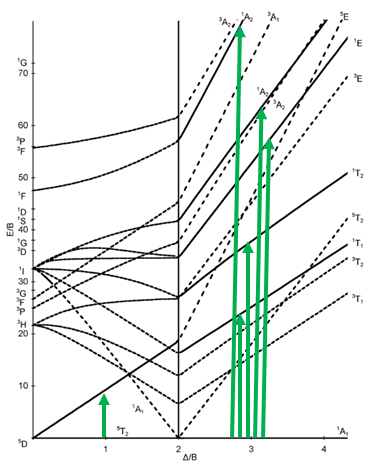
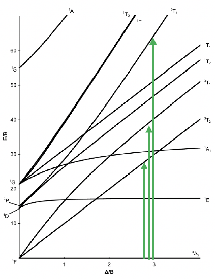
\(\newcommand{\avec}{\mathbf a}\) \(\newcommand{\bvec}{\mathbf b}\) \(\newcommand{\cvec}{\mathbf c}\) \(\newcommand{\dvec}{\mathbf d}\) \(\newcommand{\dtil}{\widetilde{\mathbf d}}\) \(\newcommand{\evec}{\mathbf e}\) \(\newcommand{\fvec}{\mathbf f}\) \(\newcommand{\nvec}{\mathbf n}\) \(\newcommand{\pvec}{\mathbf p}\) \(\newcommand{\qvec}{\mathbf q}\) \(\newcommand{\svec}{\mathbf s}\) \(\newcommand{\tvec}{\mathbf t}\) \(\newcommand{\uvec}{\mathbf u}\) \(\newcommand{\vvec}{\mathbf v}\) \(\newcommand{\wvec}{\mathbf w}\) \(\newcommand{\xvec}{\mathbf x}\) \(\newcommand{\yvec}{\mathbf y}\) \(\newcommand{\zvec}{\mathbf z}\) \(\newcommand{\rvec}{\mathbf r}\) \(\newcommand{\mvec}{\mathbf m}\) \(\newcommand{\zerovec}{\mathbf 0}\) \(\newcommand{\onevec}{\mathbf 1}\) \(\newcommand{\real}{\mathbb R}\) \(\newcommand{\twovec}[2]{\left[\begin{array}{r}#1 \\ #2 \end{array}\right]}\) \(\newcommand{\ctwovec}[2]{\left[\begin{array}{c}#1 \\ #2 \end{array}\right]}\) \(\newcommand{\threevec}[3]{\left[\begin{array}{r}#1 \\ #2 \\ #3 \end{array}\right]}\) \(\newcommand{\cthreevec}[3]{\left[\begin{array}{c}#1 \\ #2 \\ #3 \end{array}\right]}\) \(\newcommand{\fourvec}[4]{\left[\begin{array}{r}#1 \\ #2 \\ #3 \\ #4 \end{array}\right]}\) \(\newcommand{\cfourvec}[4]{\left[\begin{array}{c}#1 \\ #2 \\ #3 \\ #4 \end{array}\right]}\) \(\newcommand{\fivevec}[5]{\left[\begin{array}{r}#1 \\ #2 \\ #3 \\ #4 \\ #5 \\ \end{array}\right]}\) \(\newcommand{\cfivevec}[5]{\left[\begin{array}{c}#1 \\ #2 \\ #3 \\ #4 \\ #5 \\ \end{array}\right]}\) \(\newcommand{\mattwo}[4]{\left[\begin{array}{rr}#1 \amp #2 \\ #3 \amp #4 \\ \end{array}\right]}\) \(\newcommand{\laspan}[1]{\text{Span}\{#1\}}\) \(\newcommand{\bcal}{\cal B}\) \(\newcommand{\ccal}{\cal C}\) \(\newcommand{\scal}{\cal S}\) \(\newcommand{\wcal}{\cal W}\) \(\newcommand{\ecal}{\cal E}\) \(\newcommand{\coords}[2]{\left\{#1\right\}_{#2}}\) \(\newcommand{\gray}[1]{\color{gray}{#1}}\) \(\newcommand{\lgray}[1]{\color{lightgray}{#1}}\) \(\newcommand{\rank}{\operatorname{rank}}\) \(\newcommand{\row}{\text{Row}}\) \(\newcommand{\col}{\text{Col}}\) \(\renewcommand{\row}{\text{Row}}\) \(\newcommand{\nul}{\text{Nul}}\) \(\newcommand{\var}{\text{Var}}\) \(\newcommand{\corr}{\text{corr}}\) \(\newcommand{\len}[1]{\left|#1\right|}\) \(\newcommand{\bbar}{\overline{\bvec}}\) \(\newcommand{\bhat}{\widehat{\bvec}}\) \(\newcommand{\bperp}{\bvec^\perp}\) \(\newcommand{\xhat}{\widehat{\xvec}}\) \(\newcommand{\vhat}{\widehat{\vvec}}\) \(\newcommand{\uhat}{\widehat{\uvec}}\) \(\newcommand{\what}{\widehat{\wvec}}\) \(\newcommand{\Sighat}{\widehat{\Sigma}}\) \(\newcommand{\lt}{<}\) \(\newcommand{\gt}{>}\) \(\newcommand{\amp}{&}\) \(\definecolor{fillinmathshade}{gray}{0.9}\)Tanabe-Sugano diagrams are modified forms of correlation diagrams. The modification is simply that the energies of terms are plotted in terms of transition energy and \(\Delta\) divided by a constant, \(B\), called the Racha parameter. Terms are plotted relative to the lowest-energy term; in other words, the ground state term is plotted as the horizontal axis (\(x\)-axis). The Tanabe-Sugano diagram of a \(d^2\) transition metal complex is shown below in Figure \(\PageIndex{1}\). Tanabe-Sugano diagrams for other d-electron counts are available in the Reference Section of LibreTexts.
Tanabe-Sugano diagram of a d2 octahedral complex
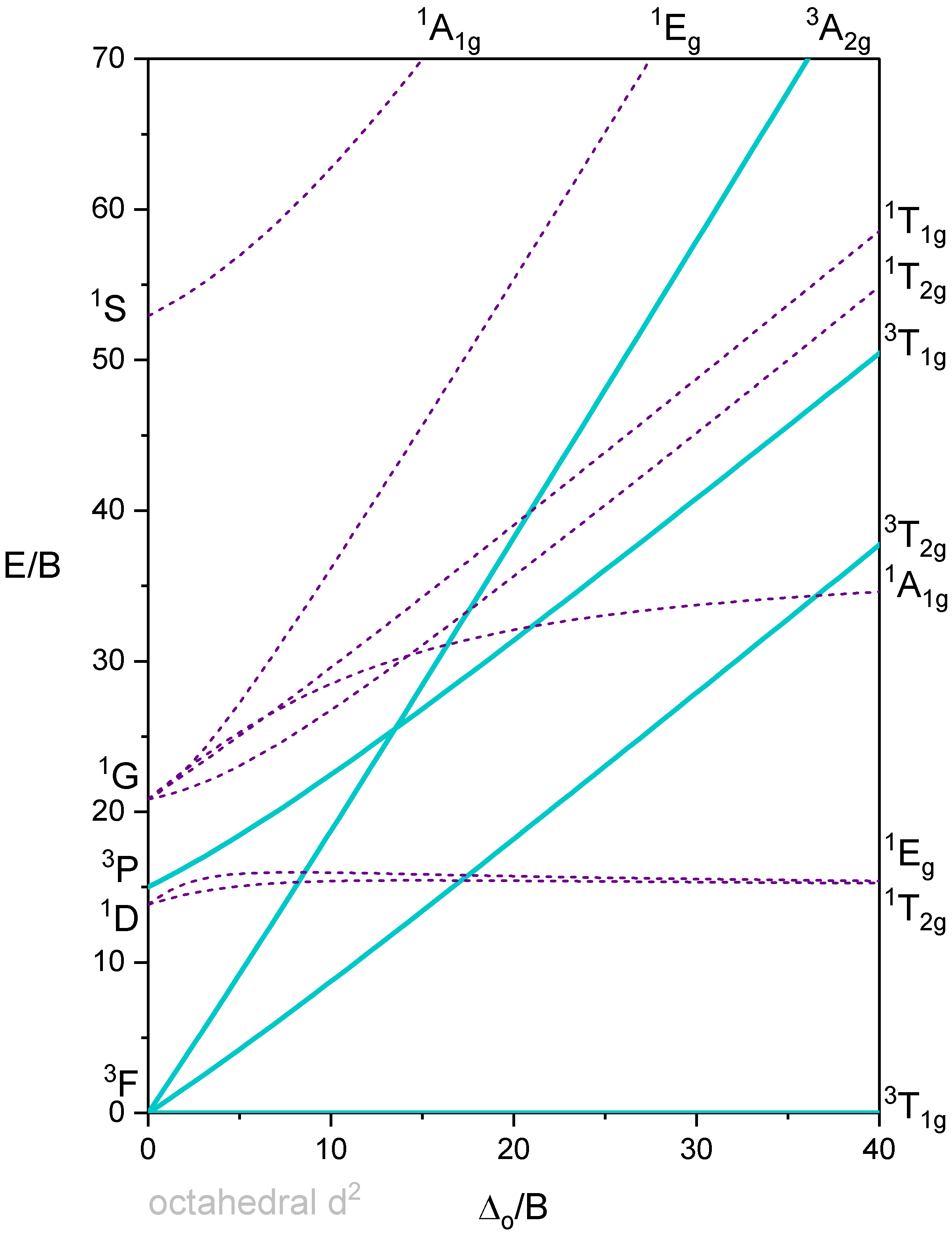
The difference between the diagram shown in Figure \(\PageIndex{1}\) and the previously-discussed correlation diagram for a \(d^2\) metal ion is that the energy of the ground state is plotted horizontally, and the energy of all other terms are plotted relative to that. In the case of the \(d^2\) electron configuration, the \(^3T_{1g}\) term is the ground term and is plotted as a horizontal line. We can see that the ligand field strength on the x-axis is given in units of B (specifically as \(\frac{\Delta}{B}\)), and the energy of the terms is also given in units of B (specifically \(\frac{E}{B}\). \(B\) is a so-called Racah parameter, which is a quantum-mechanical energy unit for the electromagnetic interactions between the electrons. It is chosen because it provides “handy” numbers.
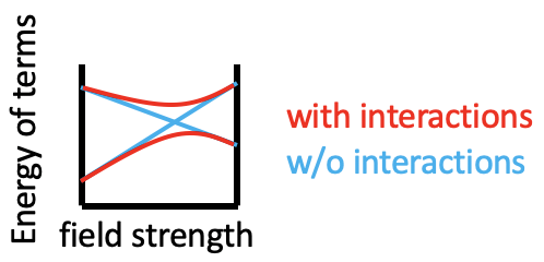
You can see that some lines in Figure \(\PageIndex{1}\) are bent (eg the two \(^1 A_{1g}\) terms), and some are straight. Bending of lines occurs when two terms interact with each other because they are close in energy and have the same symmetry. This is again an analogy to orbitals. Just as orbitals interact when they have the same symmetry type and similar energy, terms also interact when they have the same symmetry and similar energy. Without taking their interactions into account, their energies can cross when the energy of term A declines and the energy of term B increases with increasing field strength (Figure \(\PageIndex{2}\)). The closer the terms come to the point where they cross, the stronger their interactions, because their energies become more and more similar. These interactions lead to the "bending away" of the terms from each other, leading to bent curves. This means that curves for two terms of the same symmetry type will bend away in a Tanabe-Sugano diagram and never cross. For example the terms for the two \(^1 A_{1g}\) terms bend away from each other and do not cross.
Next, let us think about which electron transitions would be allowed by considering spin selection and the Laporte rule. First, notice that all the terms in Figure \(\PageIndex{1}\) have "gerade" symmetry and are labeled with a "g" subscript. In fact, this is the case for the terms of any octahedral complex. What does this mean for the allowance of electron transitions? It means that no electron transition would be allowed by the Laporte Rule, and that would imply that the complex could not absorb light. The Laporte selection rule, however, does not hold strictly. It only says that the probability of the electron-transition is reduced - but not forbidden. This means that an absorption band that disobeys the Laporte rule will have lower intensity compared to one that follows the Laporte rule, but it can still be observed. The spin-selection rule, however, holds strictly, and transitions between terms of different spin multiplicity are strictly forbidden, meaning that they have near zero probability to occur. Overall, we can therefore excite an electron from the \(^3T_1\) ground state to other triplet terms, namely the \(^3T_2\) term, and the \(^3A_2\) term (Figure \(\PageIndex{1}\)).
Tanabe-Sugano diagram of d3 octahedral complexes
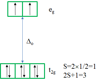
Now, let us have a look at the Tanabe-Sugano diagram of a d3 ion in an octahedral ligand field (Figure \(\PageIndex{3}\)). What is the ground term? We can see that the term designation on the horizontal line reads "\(^4A_{2g}\)”, therefore this term is the ground term. How many electron transitions from the ground state should we expect? To answer this question we need to count the number of other quartet terms. There is the \(^4T_{2g}\), the \(^4T_{1g}\), and another \(^4T_{1g}\). Thus, there are overall three electron transitions possible.
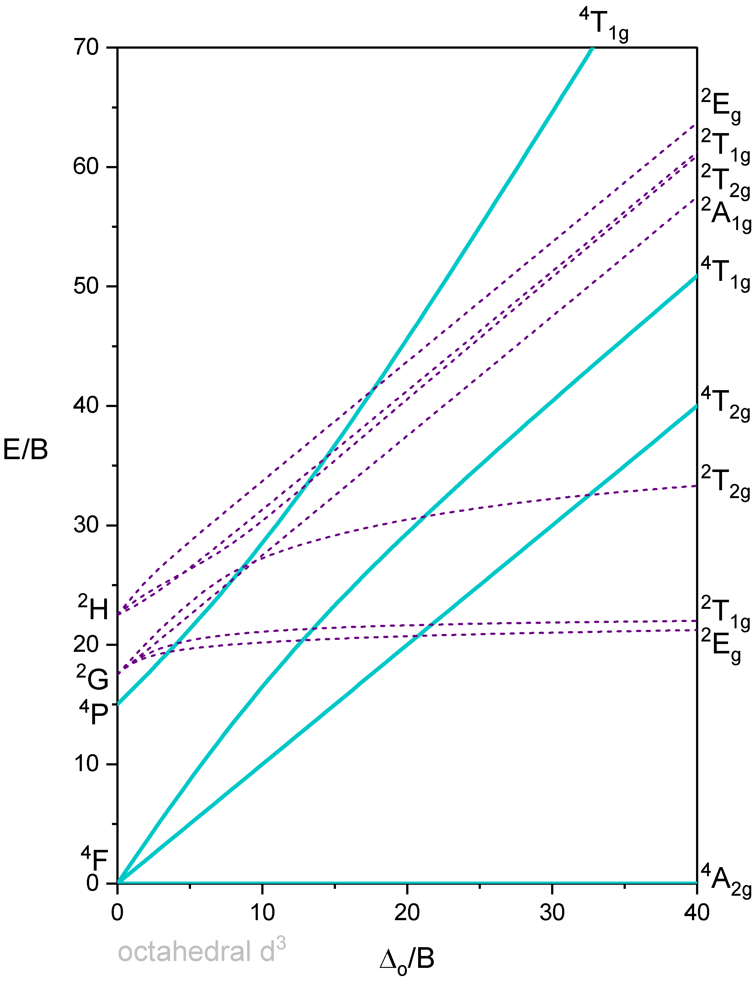
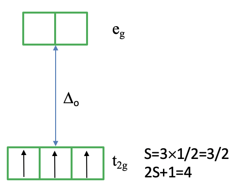
Can we understand why the ground state is a quartet term? It helps to consider how we would fill the electrons into the d-orbitals for the electron configuration d3. All three electrons would be filled spin-up in the t2g orbital following Hund’s rule (Figure \(\PageIndex{4}\)). Because each electron has the spin +1/2 the total spin of all three electrons is 3x1/2=3/2. Thus, the spin multiplicity is ((2x3/2)+1)=4. Note that the microstate we have drawn is actually only one of the (2L+1)(2S+1) microstates. S=3x1/2=3/2, but what is L? You can see on the left side of the diagram that the 4A2 term originated from a 4F term. This means L=3, and (2L+1)((2S+1)=7x4=28. This means that there are actually 27 other microstates that have the same energy as the microstate that we drew. Why did we draw this microstate in favor of the others? This is because this microstate is the state with the maximum ML (=L) and Ms (=S) values determining the term symbol.
Tanabe-Sugano diagram of d4 octahedral complexes
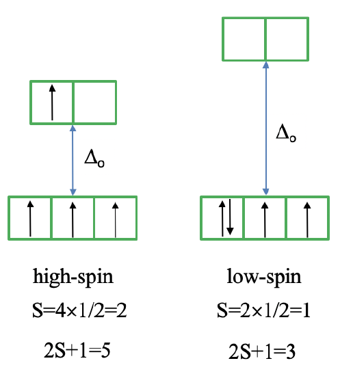
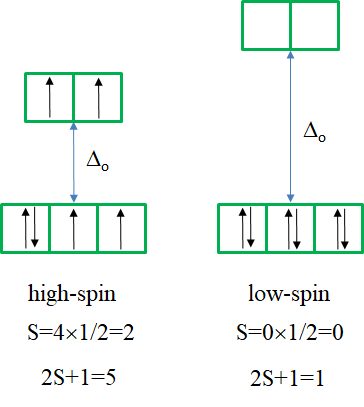
Now let us look at the Tanabe-Sugano diagram of a \(d^4\) octahedral complex (Figure \(\PageIndex{5}\)). You can see that this diagram is separated into two parts separated by a vertical line. The line indicates the ligand field strength at which the complex changes from a high spin complex to a low spin complex. At lower ligand field strengths, the ground term is a \(^5E_g\) term (solid turquoise line). At higher field strength the ground term is a \(^3T_{1g}\) term (dashed purple line).
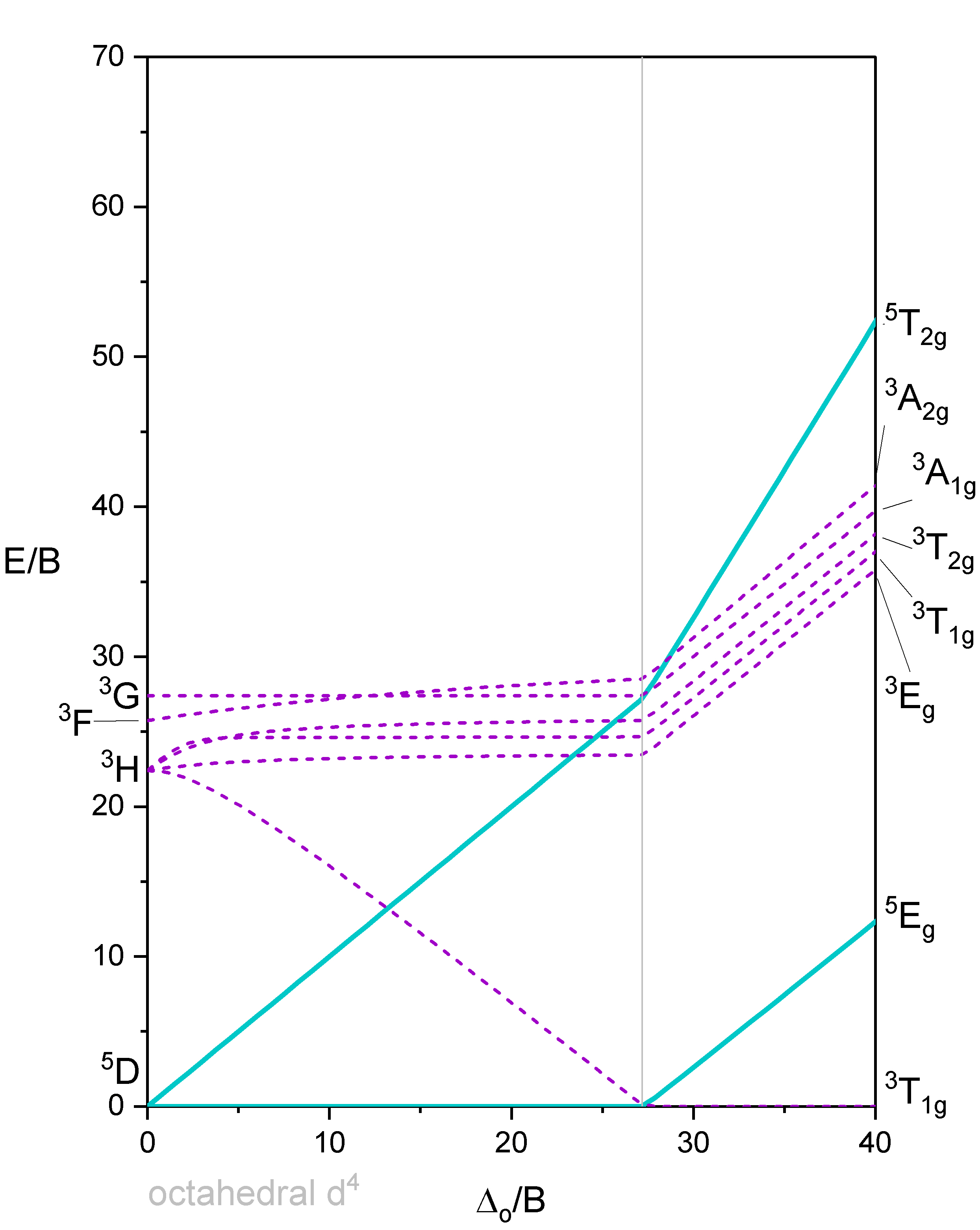
We can rationalize this again by drawing the orbital box representation of the d-orbitals in the octahedral ligand field. In the high spin state, there are four unpaired electrons, thus S=4x1/2=2, and 2S+1=5. In the low spin state, there are two unpaired electrons, and thus S=2x1/2=1, and 2S+1=3. This explains the quintet and the triplet nature of the high and low spin ground terms. Note again, that the two microstates represented by the orbital box diagrams (\(\PageIndex{6}\)) are not the only microstates that have the respective energy. They are only the "representative" microstates because they have the maximum ML and MS values.
How many electron transitions are possible from the ground term? For a high spin complex there is only one because the is only one other quintet term, namely the \(^5T_{2g}\) term. For the low spin complex, there are five transitions because there are five other triplet terms.
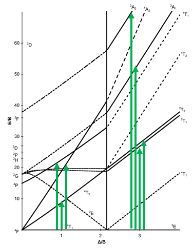
Tananbe-Sugano diagram of d5 octahedral complexes
The Tanabe-Sugano diagram of a d5 octahedral complex is also divided into two parts separated by a vertical line (Figure \(\PageIndex{7}\)). The left part reflects the high spin and the right part the low spin complex.
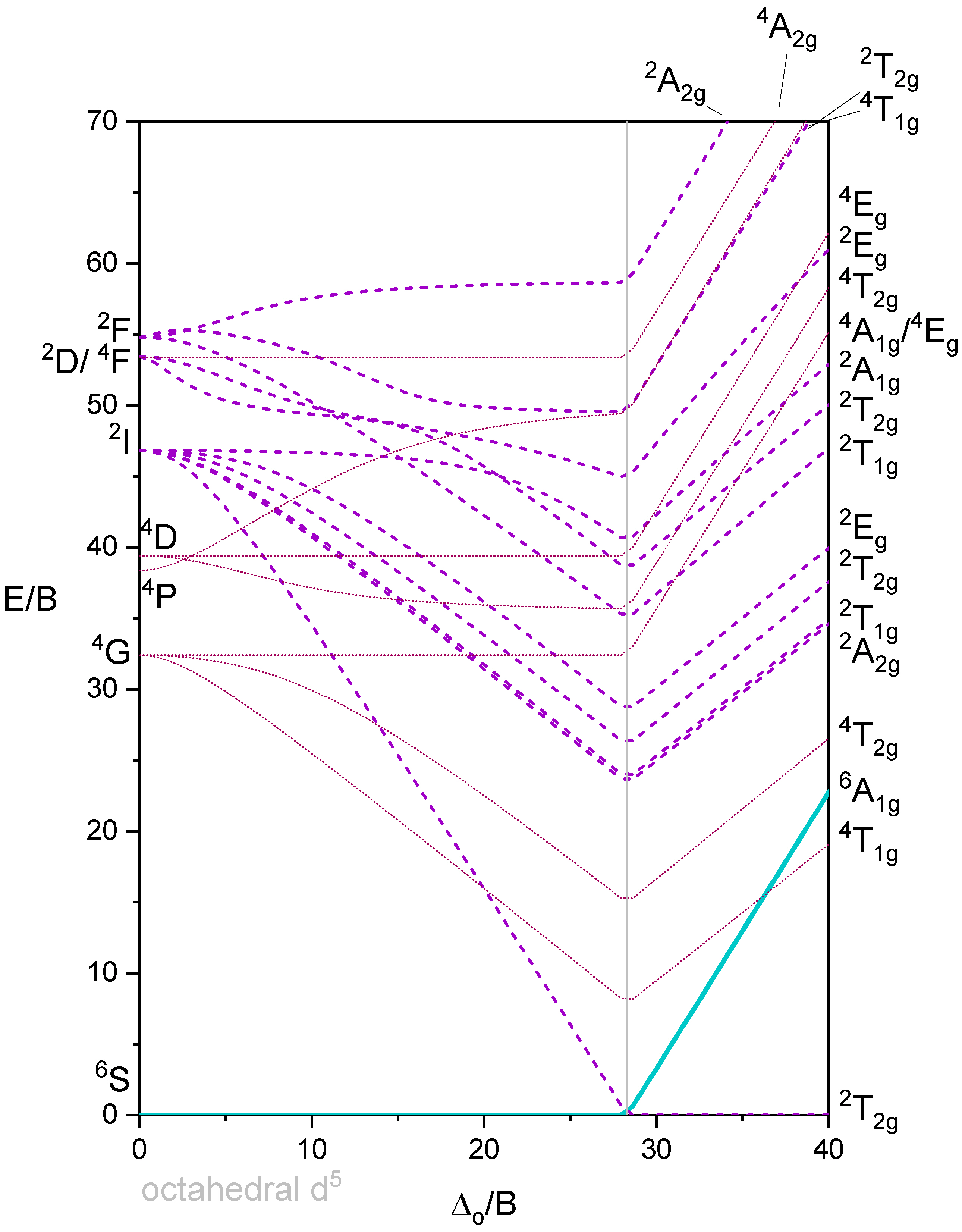
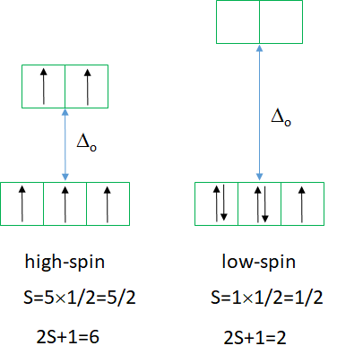
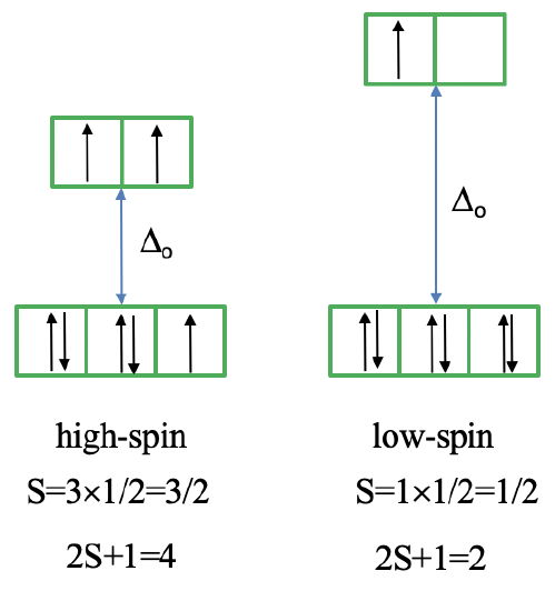
The high spin ground state is a sextet term, and the low spin ground state is a doublet term. We can understand the sextet and doublet nature of the terms when considering that the associated electron box diagrams have five and one unpaired electrons respectively. S=5x1/2=5/2 and 2S+1=6 for the high spin term, and S=1x1/2=1/2 and 2S+1=2 for the low spin term. What are the possible electron transitions from the ground state? For the high-spin complex there is no other sextet term, meaning that there is no electron transition possible. Hence, high-spin octahedral d5-complexes are colorless. An example is the hexaaqua manganese (2+) complex. A solution of this complex is near colorless, only very slightly pinkish. The slight color is because also spin-forbidden transitions can occur, albeit at a very low probability. For a d5-low spin complex there are three additional doublet states, and thus there are three electron transitions possible.
Tanabe-Sugano diagram of d6 octahedral complexes
The next diagram is the one for the d6 electron configuration (Fig. 8.2.13). Again, the diagram is separated into parts for high and low spin complexes. The dashed lines in the diagram indicate the terms that have a different spin multiplicity than the ground term. This way we can more easily see how many electron transitions are allowed.
The ground term for the high-spin complex is the quintet 5T2 term. It is a quintet term because four electrons in the d-orbitals are unpaired, and two are paired. The value for S is thus 4x1/2=2, and the spin multiplicity is 2S+1=5. The ground term for the low spin complex is a 1A1 term. It is a singlet term because all electrons are paired, and thus S=0, and 2S+1=1. How many electron transitions are there for the high-spin complex? There is only one because the 5E term is the only other quintet term. There are five transitions possible for the low-spin case because there are five additional singlet terms.
Tanabe-Sugano diagram of d7 octahedral complexes
Next, let us look at the Tanabe-Sugano diagram of a d7 octahedral complex (Fig. 8.2.15). In this case, the high spin complex has a 4T1 ground term, and the low spin complex has a 2E ground term.
The microstate that "represents" the high spin ground term has three unpaired electrons, hence the spin quantum number S=3/2 and the spin multiplicity is 2S+1=4. The microstate that represents the low spin ground term has one unpaired electron, an S value of ½, and a spin multiplicity of 2. There are three other quartet terms, and four other doublet terms, hence there are three electron transitions for the high-spin complex, and four for the low spin complex.
Tanabe-Sugano diagram of d8 octahedral complexes
Now let us look at an octahedral complex with d8 electron configuration. For this electron configuration, there are no high and low spin complexes possible, therefore, the Tanabe-Sugano diagram is no longer divided into two parts (Fig. 8.2.17).
There is a single ground term of the type 3A2. It is a triplet state because the microstate representing the term has two unpaired electrons in the eg orbitals (Fig. 8.2.18). Thus, S=2x1/2=1, and the spin multiplicity is 2S+1=2. How many electron transitions would you expect? There are three other triplet states, namely the 3T2 and two 3T1 terms. Therefore, there are three electron transitions possible.
Unnecessary diagrams for \(d^1, \; d^9, \; d^10\)
We could also ask: Are there Tanabe-Sugano diagrams for d1, d9, and d10? For, d1 there are no electron-electron interactions, thus the simple orbital picture is sufficient. The 2D term splits into T2g and Eg terms, and there is only one electron transition possible. The d9 electron configuration is the “hole-analog” of the d1 electron configuration. It has also just one 2D term which splits into a T2g and an Eg term in the octahedral ligand field. Therefore, also in this case there is only one electron transition from the T2g into the Eg term possible. In the case of d10 all microstates are filled with orbitals, and there is only the 1S term which does not split in an octahedral ligand field. Therefore, there are no electron transitions in this case.
Jahn-Teller distortions and other geometries
Some of the electron configurations discussed above are ones that are particularly susceptible to Jahn-Teller distortion. The Jahn-Teller theorem predicts that electron configurations with asymmetrically populated orbitals (i.e., those that have spin multiplicity of a doublet or greater), will distort. Distortions affect the electronic spectra of coordination complexes, and in practice Jahn-Teller distortions are significant only in the cases where the \(e_g\) orbitals are asymmetrically populated (e.g., octahedral \(d^9\) and high spin \(d^4\)).
Finally, it should be mentioned that it is also possible to construct Tanabe-Sugano diagrams for other shapes such as the tetrahedral shape, but we will not discuss these further here.
Dr. Kai Landskron (Lehigh University). If you like this textbook, please consider to make a donation to support the author's research at Lehigh University: Click Here to Donate.