2.2.2: Quantum Numbers and Atomic Wave Functions

The one-dimensional particle in a box model from the previous section shows us how a wavefunction works in one dimension (the x- dimension). In one dimension, the wavefunction requires only one quantum number, \(n\). A full explanation of the three-dimensional wavefunction for an electron is outside of the scope of this course. Instead, we will focus on gaining a conceptual understanding by extending knowledge of the one-dimensional wavefunction to a three-dimensional space.

Quantum numbers

Extending the wavefunction to three dimensions requires a total of three quantum numbers. In addition to \(n\), which we saw in the one-dimensional case, we also need \( l\) and \(m_l\) to express the wavefunction in three dimensions. A complete solution to the Schrödinger equation, both the three-dimensional wavefunction and energy, includes a set of three quantum numbers (\(n, l, m_l\)). The wavefunction describes what we know as an atomic orbital; it defines the region in space where the electron is located. Additionally, there is a fourth quantum number, \(m_s\). The \(m_s\) quantum number accounts for the observed interaction of electrons with an applied magnetic field; it is an additional postulate that is not part of the wavefunction. These four quantum numbers are described below.

The quantum number, \(n\): This is the principle quantum number. This number represents the shell, including both the overall energy of the electron in that shell and the size of that shell. An allowed value for \(n\) is any non-zero, positive integer (1, 2, 3, 4, ... etc are allowed, but 4.1 is not allowed).

The quantum number, \(l\): This is the angular momentum quantum number that corresponds to the subshell and its shape. It represents the angular dependence of the subshell, or the "shape" of the orbitals within a subshell. The allowed values of \(l\) depend on \(n\). The allowed values of \(l\) for an electron in shell \(n\) are integer values between \(0\) to \(n-1\), or \(l = 0\rightarrow n-1\). These values correspond to the orbital shape where \(l=0\) is an s-orbital, \(l=1\) is a p-orbital, \(l=2\) is a d-orbital, and \(l=3\) is an f-orbital.

The quantum number \(m_l\): This is the magnetic quantum number. Its possible values give the number of orbitals within a subshell and its specific value gives the orbital's orientation in space. The allowed values of \(m_l\) depend on the value of \(l\). The value of \(m_l\) is allowed to be any positive or negative integer between \(+l\) and \(-l\). In other terms, \(m_l=+l \rightarrow -l\). For example, if the electron is in a 3-p-orbital, then \(n=3, l=1\), and the possible values of \(m_l\) are \(-1, 0,\) and \(+1\). Since there are three possible values of \(m_l\) there are three orbitals in the \(p\) subshell. The specific \(m_l\) value defines in which of the three possible p-orbitals (\(p_x, p_y,\) or \(p_z\)) the electron exists. In the case of the \(s\) subshell, there is only one value, \(m_l=0\) because \(l=0\). The one value corresponds to the fact that there is only one \(s\) orbital in any shell.

The quantum number \(m_s\): This quantum number accounts for the electron's "spin". In short, electrons interact with magnetic fields in a way that is similar to how a tiny bar magnet would interact with a magnetic field. The allowed values for \(m_s\) are \(+\frac{1}{2}\) and \(-\frac{1}{2}\).

Table \(\PageIndex{1}\). Quantum Numbers

SYMBOL	NAME	VALUES	MEANING
\(n\)	principal	\(1,2,3...\)(any integer)	energy level, shell
\(l\)	angular momentum	\(0 \rightarrow n-1\)	subshell, \(0=s, 1=p, 2=d, 3=f...\) this is the angular dependence of the orbital, shape of the orbital *letters have historical meaning, sharp, principle, diffuse, fundamental
\(m_l\)	magnetic	\(+l \rightarrow -l\)	orientation of angular momentum in space, orbital
\(m_s\)	spin	\(+\frac{1}{2}, -\frac{1}{2}\)	the imaginary property we call "spin", up or down

1-Electron Wavefunctions (Atomic orbitals)

One simplified representation of the three-dimensional wavefunction is shown below. This representation breaks the wavefunction into two parts: the radial contribution (\(\textcolor{blue}{R_{n,l}(r)}\)) and the angular contribution (\(\textcolor{red}{Y_{l,m_l}(\theta,\phi)}\)).

\[\psi_{(n,l,m_l)}= \textcolor{blue}{R_{n,l}(r)} \times \textcolor{red}{Y_{l,m_l}(\theta,\phi)} \label{WF1} \]

Allowed Energies

From the wavefunction, we can find the allowed energies of an electron in an atom. We have not given you the more complex form of the wavefunction where you'd need to derive \ref{E} from \ref{WF1} because it is outside the scope of this course. Instead, consider the process that we used to derive the energy of a particle in a one-dimensional box in the previous section. A similar process can be used to find the energy of an electron in three dimensions, shown in \ref{E}.

\[E_n = -\frac{hcRZ^2}{n^2}=-(13.607\thinspace eV) \left(\frac{Z}{n}\right)^2 \label{E} \],

where \(n\) is the principle quantum number, \(h\) is Planck's constant, \(c\) is the speed of light, \(R\) is the Rydberg constant, and \(Z\) is the charge of the nucleus. It is useful to know that the value of \(hcR = 13.6 eV\). This is also the value of the ionization energy of an electron in a hydrogen atom. This equation only works for hydrogenic atoms (atoms or ions that are "like" hydrogen in that they have only one electron).

Exercise \(\PageIndex{1}\)

The energy that it takes to eject a ground-state electron from a hydrogen atom (its ionization energy, IE) is measured to be approximately 13.6 eV, while the IE energy of a He⁺ ion is four times greater at 54.4 eV. These values can be predicted using both Equation \ref{E} and the Rydberg equation.

1. Using Equation \ref{E} for allowed energies of electrons in a hydrogen atom, derive the energy of the ground state electron in H. Then repeat this process for a He⁺ ion. What do the values indicate about the relative attraction between an electron and the nuclei of these two hydrogenic atoms?
2. Show that the IE of H's 1s electron can also be predicted by the Rydberg formula (equation 2.1.2.2).

Answer (a)

Use Equation \ref{E} . For a hydrogen atom with one proton, \(Z=1\), and the ground state energy level is the lowest energy level, \(n=1\). Therefore, the energy of an electron in the ground state of a H atom is:

\(E_n = -\frac{hcRZ^2}{n^2} = -13.607\thinspace eV(\frac{1}{1})^2 = -13.607 \thinspace eV \), or approximately \(-13.6 \thinspace eV\). Thus, the IE (energy necessary to remove that electron) is +13.6 eV.

We can use the same process to find the ground state energy of an electron in He⁺. This time, \(Z=2\) because helium has two protons in its nucleus, and as before, the ground state is \(n=1\).

\(E_n = -\frac{hcRZ^2}{n^2} = -13.607\thinspace eV(\frac{2}{1})^2 = -54.428 eV \), or approximately \(-54.4 \thinspace eV\). Thus, the IE is +54.4 eV.

These ground-state energies are the same as the energy required to remove the ground state electron from H and He⁺. In other words, these are the predicted ground state IE values for one electron in H and He⁺. The measured IEs for these two species are in fact 13.6 eV and 54.4 eV, respectively.

The He⁺ ion has a more negative value for its ground state energy with a magnitude four times greater than that of the ground state H electron. This means that the He⁺ electron is more strongly attracted to the (+2) nucleus than the H electron is attracted to the (+1) nucleus, and more energy is required to eject the He⁺ electron than the H electron. It takes more energy to remove the electron from He⁺ than from H. This makes sense in light of Coulomb's law: The attractive force between the H nucleus (+1) and an electron (-1) would be weaker than that of a He nucleus (+2) and an electron (-1) because the positive charge of the He nucleus has a greater magnitude.

Answer (b)

The Rydberg equation is: \( \dfrac{1}{\lambda }= E (cm^{-1})= R_H\; \left ( \dfrac{1}{n_l^{2}}-\dfrac{1}{n_h^{2}} \right )\) where \(n_l\) and \(n_h\) are positive integers, \(n_h > n_l\), and the Rydberg constant (\(R_H\)), has a value of 1.09737 × 10⁷m⁻¹. We should set \(n_l=1\) to represent the initial ground state, and \(n_h=\infty\) to represent the removal of the electron from the atom.

Step 1.

Calculate Energy (in m^-1) using the Rydberg equation:

\(E = R_H\left( \dfrac{1}{n_l^{2}}-\dfrac{1}{n_h^{2}} \right) = 1.09737\times10^7 m^{-1} \left( \dfrac{1}{1^{2}}-\dfrac{1}{\infty^{2}} \right ) = 1.09737\times10^7 m^{-1} \left( 1-0 \right ) = 1.09737 \times 10^7 m^{-1}\)

Ultimately, we want a value of energy in units of eV so we can compare it to the answers in part (a), but our value here is in units of inverse meters (m^-1). A quick internet search can tell you the conversion between inverse centimeters (cm^-1) and eV is \(1 eV = 8065.6 cm^{-1}\).

Step 2.

Convert from m^-1 to cm^-1 to eV so that we can compare to the answer in part (a):

\(1.09737\times 10^7 \frac{1}{m} \times \dfrac{1m}{100cm} \times \dfrac{1eV}{8065.6 \frac{1}{cm}} = 13.6056 eV,\) or approximately 13.6 eV.

Exercise \(\PageIndex{2}\)

Which of the following are hydrogenic atoms? H, H⁺, H^-, He, He²⁺, He⁺, He^-, Li, Li³⁺, Li²⁺, Li⁺, Li^- .

Answer

Hydrogenic atoms are atoms or ions that contain only one electron. H, He⁺, and Li²⁺ are hydrogenic atoms/ions that contain only one electron.

Radial and Angular contributions to the wavefunction:

Radial contribution, \(\textcolor{blue}{R_{n,l}(r)}\)

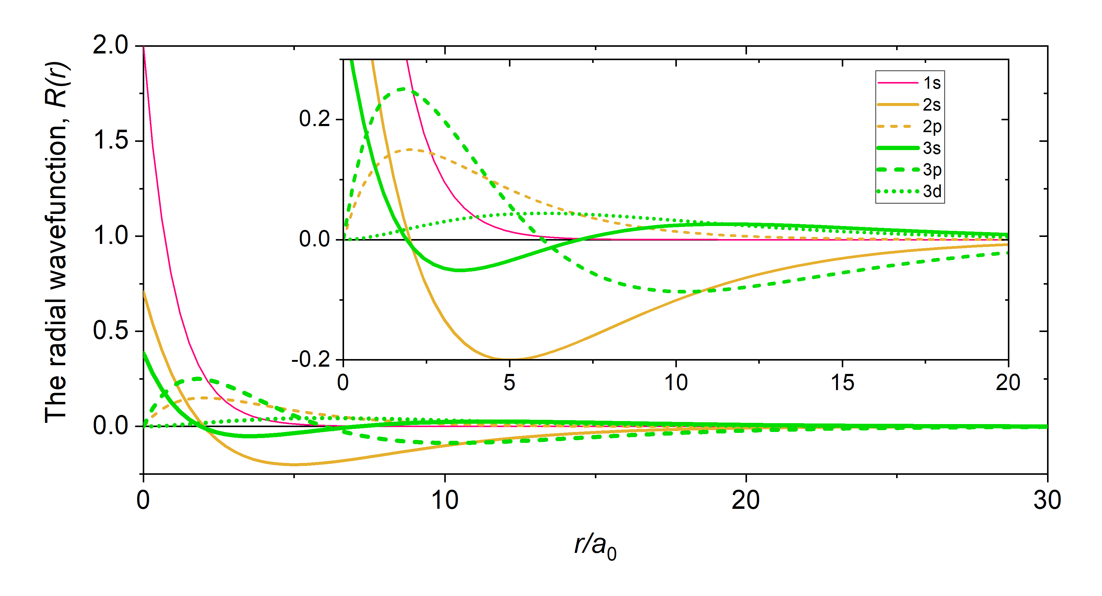
The radial part of the wavefunction, \(\textcolor{blue}{R_{n,l}(r)}\) gives the radial variation of \(\psi\). In other words, \(\textcolor{blue}{R_{n,l}(r)}\) defines how the wavefunction depends on the distance of the electron from the nucleus (the radius). The \(\textcolor{blue}{R_{n,l}(r)}\) parts of the wavefunction for a hydrogenic atom are listed in Table \(\PageIndex{2}\), and they are plotted in Figure \(\PageIndex{1}\). Notice that the \(R_{n,l}(r)\) of all s-orbitals (solid lines) reaches a maximum at \(r=0\). This is unique to the s-orbitals' \(R_{n,l}(r)\). The \(R_{n,l}(r)\) of p- and d-orbitals orbitals approaches zero as r approaches zero. This has important consequences for how closely an electron in these orbitals can approach the nucleus.

Figure \(\PageIndex{1}\). Plots of the radial wavefunction, \(\textcolor{blue}{R_{n,l}(r)}\), for the first three shells. The wavefunctions are plotted relative to \(\dfrac{r}{a_0}\), where \(a_0 = 52.9 pm = 0.529 Å\) is the Bohr Radius (the radius of a hydrogen 1s orbital). The expressions for these radial wavefunctions (\(\textcolor{blue}{R_{n,l}(r)}\)) are shown in Table \(\PageIndex{2}\). (Kathryn Haas; CC-NC-BY-SA)

Table \(\PageIndex{2}\). Radial wavefunctions (\(R(r)\)) for the first three shells of a hydrogen atom. \(Z\) is the nuclear charge, and \(a_0 = 52.9 pm = 0.529 Å\) is the Bohr radius (the radius of a hydrogen 1s orbital). For the H atom, \(Z=1\) (the nuclear charge of hydrogen). Plotting of the functions can be simplified if we set \(a_0=1\) and plot the functions with respect to \(r/a_0\), which was done to find the plots shown in Figure \(\PageIndex{1}\).

Orbital	\(n\)	\(l\)	\(\textcolor{blue}{R_{n,l}(r)}\)
1s	1	0	\(2\left[\frac{Z}{a_0}\right]^{3/2}e^{-Zr/a_0}\)
2s	2	0	\(2\left[\frac{Z}{2a_0}\right]^{3/2}\left(2-\frac{Zr}{a_0}\right)e^{-Zr/2a_0}\)
2p	2	1	\(\frac{1}{\sqrt{3}}\left[\frac{Z}{3a_0}\right]^{3/2}\left(\frac{Zr}{a_0}\right)e^{-Zr/2a_0}\)
3s	3	0	\(\frac{2}{27}\left[\frac{Z}{3a_0}\right]^{3/2}\left(27-18\frac{Zr}{a_0}-2(\frac{Zr}{a_0})^2\right)e^{-Zr/3a_0}\)
3p	3	1	\(\frac{1}{81\sqrt{3}}\left[\frac{2Z}{a_0}\right]^{3/2}\left(6-\frac{Zr}{a_0}\right)(\frac{Zr}{a_0})e^{-Zr/3a_0}\)
3d	3	2	\(\frac{1}{81\sqrt{15}}\left[\frac{2Z}{a_0}\right]^{3/2}\left(\frac{Zr}{a_0}\right)^2e^{-Zr/3a_0}\)

Radial probability function, \(\textcolor{black}{4 \pi r^2}\textcolor{blue}{(R_{n,l}(r))^2}\)

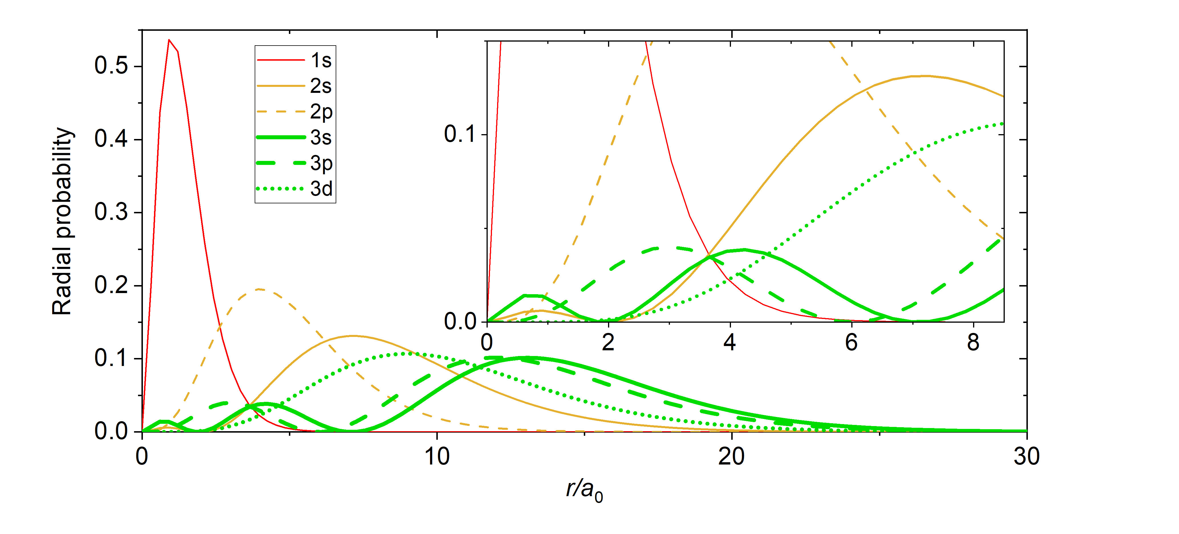
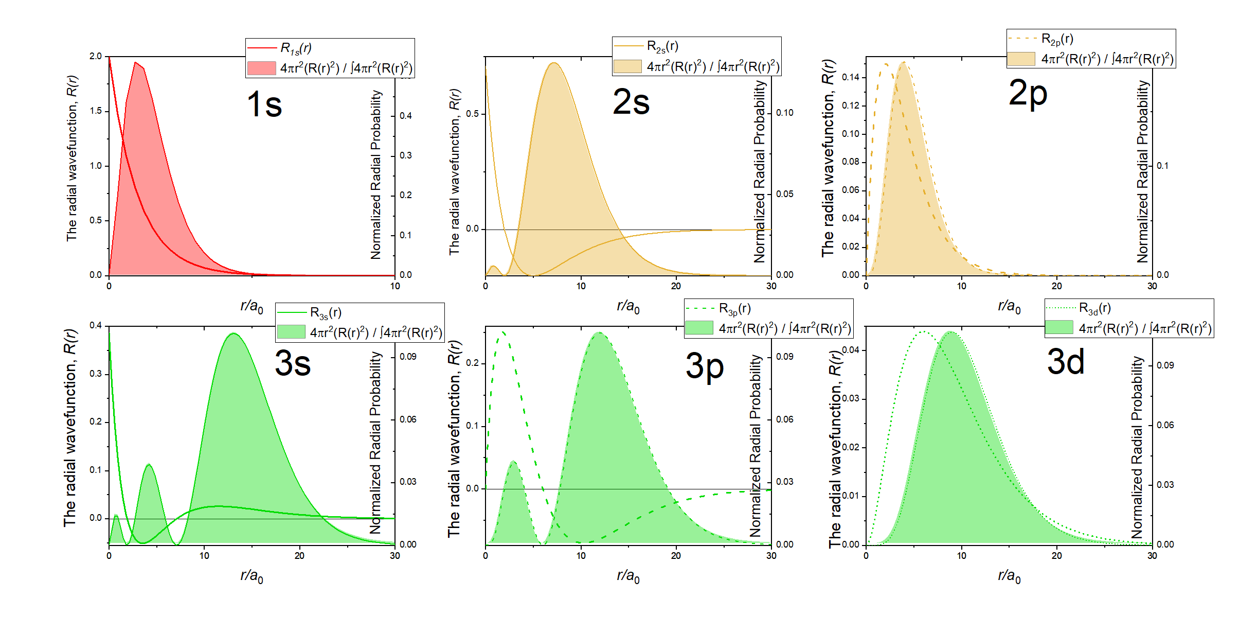
Just like in the particle-in-a-box model, the square of the wavefunction is proportional to the probability of finding a particle (electron) at some point in space. The square of the radial part of the wavefunction is called the radial distribution function \(4 \pi r^2\textcolor{blue}{(R_{n,l}(r))^2}\), and it describes the probability of locating the electron at some distance \(r\) away from the nucleus. When we normalize the probability functions by dividing the function by its integral over all space, we get the plots shown in Figure \(\PageIndex{2}\). The normalized probability functions are compared to the original radial part of the wavefunctions in Figure \(\PageIndex{3}\). The most probable distance for finding an electron is shown by the maximum value of the function. For an electron in the 1s orbital of H, the most probable distance from the nucleus occurs at \(r=1a_0\). This is the Bohr Radius, and it has a value of \(a_0 = 52.9 pm = 0.529 Å\). It is convenient to plot the functions of the hydrogen atomic orbitals relative to the size of its smallest orbital, the 1s orbital; this is the reason we plot \(R_{n,l}(r)\) and \(4 \pi r^2(R_{n,l}(r))^2\) relative to \(\frac{r}{a_0}\).

Figure \(\PageIndex{2}\): Plots of the normalized radial probability functions for the first three shells. The radial wavefunctions (\(\textcolor{blue}{R_{n,l}(r)}\)) are shown in Table \(\PageIndex{2}\). (Kathryn Haas; CC-NC-BY-SA)

Figure \(\PageIndex{2}\). Plots of the normalized radial probability function for each orbital in the first three shells (shaded curves). The radial wavefunctions are also shown (Table \(\PageIndex{2}\)). The y-axis on the left of each plot corresponds to the radial wavefunction (line); the y-axis on the right of each plot corresponds to the radial probability function (shaded). (Kathryn Haas; CC-NC-BY-SA)

Radial nodes

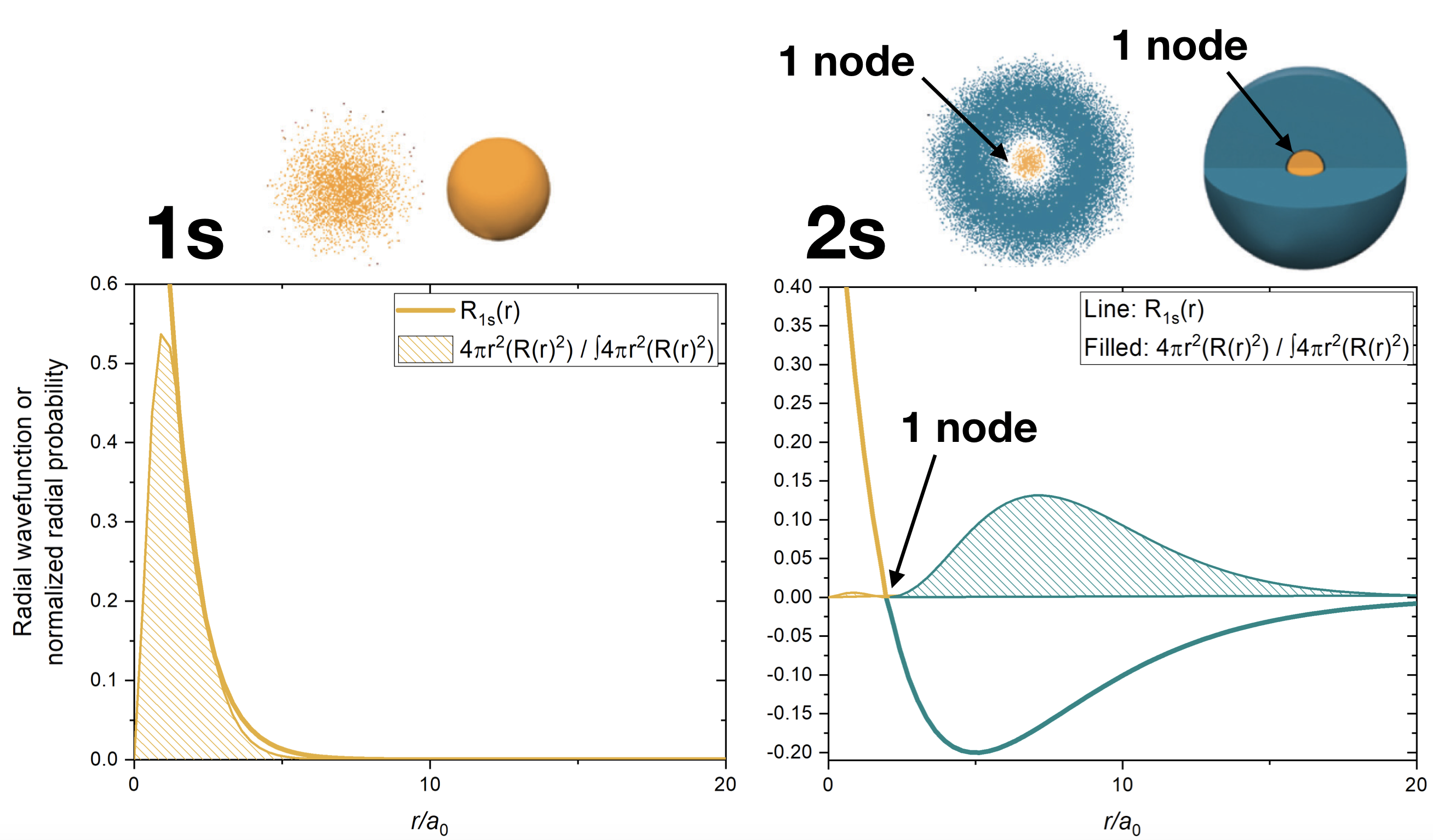
From the discussion of the 1-dimensional particle in a box, we learned that nodes exist where \(\psi=0\). In the case of the 3-dimensional wavefunction, there are two different types of nodes: radial nodes and angular nodes. Radial nodes occur where the radial part of the wavefunction is zero (\(R(x)=0\)). These are easy to find by plotting the radial part of the wavefunction and finding where the radial part of the wavefunction (and the radial probability function) is zero (where \(\textcolor{blue}{R_{n,l}(r)}=0\)) and where \(4 \pi r^2\textcolor{blue}{(R_{n,l}(r))^2}=0\). These nodes are spherical in shape and depend on the energy level and subshell (the values of \(n\) and \(l\)). The number of radial nodes is \(n-l-1\). An example of a radial node is the single node that occurs in the \(2s\) orbital (\(2-0-1=1\) node). In contrast, the 1s orbital has zero radial nodes (\(1-0-1=0\) nodes). Where there is a node, there is zero probability of finding an electron.

Figure \(\PageIndex{3}\): Visualization of the 1s and 2s atomic orbitals. Each orbital is shown as both an electron probability density plot and a contour plot above its wavefunction and probability density function. The 1s orbital has zero radial nodes. The 2s orbital has one radial node where its wavefunction changes sign and its radial probability function is zero. (Kathryn Haas; CC-BY-SA)

Boundary surfaces

A true node occurs where the probability of finding an electron is zero. Nodes occur where \(\psi=\psi^2=0\). Far from the nucleus, the probability of finding the electron rapidly approaches zero, but is never exactly zero. What this means is that it is rather improbable to find the electron at far distances from the nucleus, but it's not impossible. The rapid fall of probability creates a boundary surface rather than a node. The boundary surface represents the area around the nucleus where the electron exists most of the time.

Exercise \(\PageIndex{1}\)

How many radial nodes are in the s, p, d, and f orbitals in the first four shells? \(n=1,2,3,4\)?

Answer

You can approach this answer by using the mathematical relationship between the number of radial nodes and the values of \(n\) and \(l\): number of radial nodes is \(n-1-l\). You could also notice the pattern that the first orbital of any type (1s, 2p, 3d...) has zero radial nodes, the second orbital of a type (2s, 3p, 4d...) has one radial node, the third orbital of a type has two radial nodes (3s, 4p, 5d...)...etc.

A full list of all of the orbitals in the first four shells and their number of radial nodes is below. It's a good idea to prove to yourself that the numbers given below are consistent with the plots of the orbitals' wavefunctions for those orbitals in the first three shells:

s-orbitals:

1s: \(n-1-l = 1-1-0 = 0\), zero radial nodes

2s: \(n-1-l = 2-1-0 = 1\), one radial node

3s: \(n-1-l = 3-1-0 = 2\), two radial nodes

4s: \(n-1-l = 4-1-0 = 3\), three radial nodes

p-orbitals

2p: \(n-1-l = 2-1-1 = 0\), zero radial nodes

3p: \(n-1-l = 3-1-1 = 1\), one radial node

4p: \(n-1-l = 4-1-1 = 2\), two radial nodes

d-orbitals

3d: \(n-1-l = 3-1-2 = 0\), zero radial nodes

4d: \(n-1-l = 4-1-2 = 1\), one radial nodes

f-orbital

4f: \(n-1-l = 4-1-3 = 0\), zero radial nodes

Exercise \(\PageIndex{1}\)

Draw a rough plot of the following:

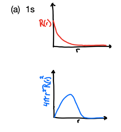
1. The radial wavefunction, \(R_{n,l}(r)\) and the probability density function, \(4 \pi r^2(R_{n,l}(r))^2\), for the 1s orbital.
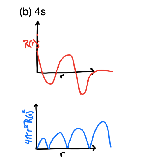
2. The radial wavefunction, \(R_{n,l}(r)\) and the probability density function, \(4 \pi r^2(R_{n,l}(r))^2\), for the 4s orbital.

Answer, 1s

The 1s orbital's \(R_{n,l}(r)\) reaches a maximum near the origin and approaches zero far from the nucleus. The \(4 \pi r^2(R_{n,l}(r))^2\) approaches zero at the origin, has a maximum intensity at the Bohr radius, and approaches zero far from the nucleus (its boundary surface).

.

Answer, 4s

Like all s orbitals, the 4s orbital's \(R_{n,l}(r)\) reaches a maximum near X=0, but it would be less intense than the function of the 1s, 2s, and 3s orbitals. It should have three radial nodes and so its wavefunction would change sign three times. This would give four regions of electron density in the probability function while the function would approach zero (boundary surface) far from the nucleus.

Angular contribution, \(\textcolor{red}{Y_{l,m_l}(\theta,\phi)}\), and angular probability function, \(\textcolor{red}{(Y_{l,m_l}(\theta,\phi))^2}\)

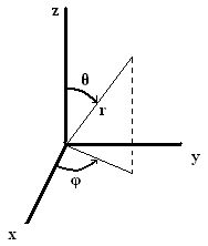The angular contribution to the wavefunction, \(\textcolor{red}{Y_{l,m_l}(\theta,\phi)}\), describes the wavefunction's shape, or the angle with respect to a coordinate system. To describe the direction in space, we use spherical coordinates that tell us distance and orientation in 3-dimensional space. There are three spherical coordinates: \(r, \phi,\) and \(\theta\). \(r\) is the radius, or the actual distance from the origin. \(\phi\) and \(\theta\) are angles. \(\phi\) is measured from the positive x axis in the xy plane and may be between 0 and \(2\pi\). \(\theta\) is measured from the positive z axis towards the xy plane and may be between 0 and \(\pi\).

\[\textcolor{red}{Y_{l,m_l}(\theta,\phi)}=\left ( \dfrac{1}{4\pi} \right )^{1/2}y\left (\theta,\phi \right ) \nonumber \]

\(\textcolor{red}{Y_{l,m_l}(\theta,\phi)}\), is slightly more difficult to describe than the radial contribution was. This is partly because \(\textcolor{red}{Y_{l,m_l}(\theta,\phi)}\) contains imaginary numbers, which have no real, physical meaning. However, the angular part of the wavefunction becomes more "real" when you square it to get angular probability density, a more tangible concept described as the shapes of orbitals.

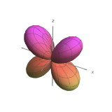
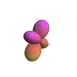
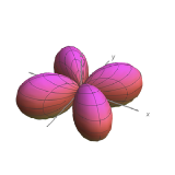
The values of \(\theta\), \(\phi\), and \(y(\theta,\phi)\) for orbitals in the hydrogen atom are listed in Table \(\PageIndex{3}\). But \(Y_{l,m_l}(\theta,\phi)\) is only a mathematical function and has no real physical meaning. The square of the radial wavefunction, \(Y_{l,m_l}(\theta,\phi)^2\), gives the probability of finding the electron at a point in space on a ray described by \((\phi, \theta)\). Thus \(Y_{l,m_l}(\theta,\phi)^2\) describes the shape of the orbital.

Table \(\PageIndex{3}\). Components of the angular wavefunction and the resulting orbital shapes. The plots in the two right hand columns were created using Desmos and Mathematica: specifically "Spherical Harmonics" from the Wolfram Demonstrations Project, http://demonstrations.wolfram.com/SphericalHarmonics/ and "Visualizing Atomic Orbitals" demonstrations.wolfram.com/Vi...tomicOrbitals/.

subshell	\(m_l\) (orbital)	\(\theta\)	\(\phi\)	Plots of \(\theta^2\)	orbital shapes
\(l=0\), s	\(m_l=0\)	\(\frac{1}{\sqrt{2}}\)	\(\frac{1}{\sqrt{2 \pi}}\)
\(l=1\), p	\(m_l=0\)	\(\frac{\sqrt{6}}{2} \cos \theta\)	\(\frac{1}{\sqrt{2 \pi}}\)
\(l=1\), p	\(m_l=+1\)	\(\frac{\sqrt{3}}{2} \sin \theta\)	\(\frac{1}{\sqrt{2 \pi}} e^{i \phi}\)
\(l=1\), p	\(m_l=-1\)	\(\frac{\sqrt{3}}{2} \sin \theta\)	\(\frac{1}{\sqrt{2 \pi}} e^{-i \phi}\)
\(l=2\), d	0	\(\frac{\sqrt{10}}{4}\left(3 \cos ^{2} \theta-1\right)\)	\(\frac{1}{\sqrt{2 \pi}}\)
\(l=2\), d	\(m_l=+1\)	\(\frac{\sqrt{15}}{2} \sin \theta \cos \theta\)	\(\frac{1}{\sqrt{2 \pi}} e^{i \phi}\)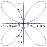
\(l=2\), d	\(m_l=-1\)	\(\frac{\sqrt{15}}{2} \sin \theta \cos \theta\)	\(\frac{1}{\sqrt{2 \pi}} e^{-i \phi}\)
\(l=2\), d	\(m_l=+2\)	\(\frac{\sqrt{15}}{4} \sin ^{2} \theta\)	\(\frac{1}{\sqrt{2 \pi}} e^{i 2 \phi}\)
\(l=2\), d	\(m_l=-2\)	\(\frac{\sqrt{15}}{4} \sin ^{2} \theta\)	\(\frac{1}{\sqrt{2 \pi}} e^{-i 2 \phi}\)

Angular nodes

Angular nodes exist where \(\textcolor{red}{(Y_{l,m_l}(\theta,\phi))^2}=0\). These nodes are planar in shape, and they depend on the value of \(l\). The number of angular nodes in any orbital is equal to \(l\). This means that s-orbitals (\(l=0\)) have zero angular nodes, p-orbitals (\(l=1\)) have one angular node, d-orbitals (\(l=2\)) have two angular nodes, and so on. Planar nodes can be flat planes (like the nodes in all p orbitals) or they can have a conical shape, like the two angular nodes in the \(d_{Z^2}\) orbital. Angular nodes in some p and d orbitals are shown in Figure \(\PageIndex{4}\).

Figure \(\PageIndex{4}\): The angular nodes in p-orbitals and d-orbitals are shown. Every p orbital has one angular node, and every d orbital has two angular nodes. The number of angular nodes in any orbital is equal to the value of the quantum number, \(l\). (CC BY-NC-SA; anonymous by request)

Atomic Orbitals

Atomic orbitals result from a combination of both the radial and angular contributions of the wavefunction. Atomic orbitals can have both angular nodes and radial nodes, depending on the values of \(n\) and \(l\).

The chart below compares the radial variation, angular variation, and their combinations (orbitals).

Orbital	Radial Probability	Radial Nodes	Angular Probability	Angular Nodes	Combination (Orbital)	Total Nodes
1s		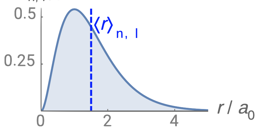0		0		0
2s		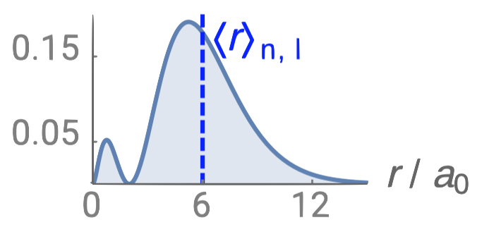1		0		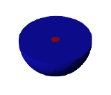1
2p		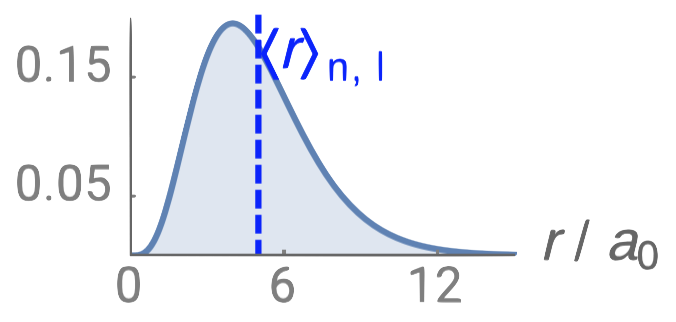0		1		1
3s		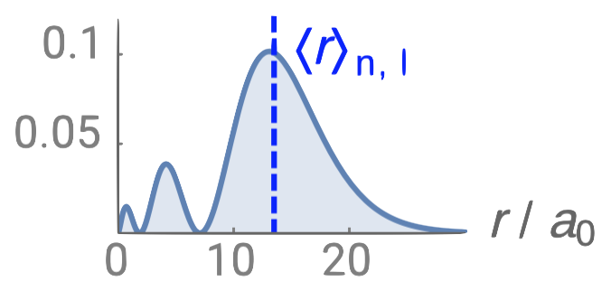2		0		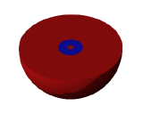2
3p		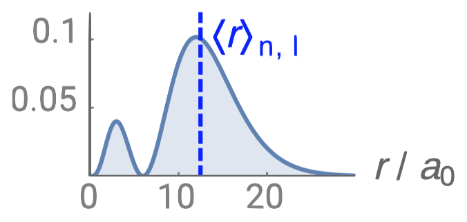1		1		2
3d		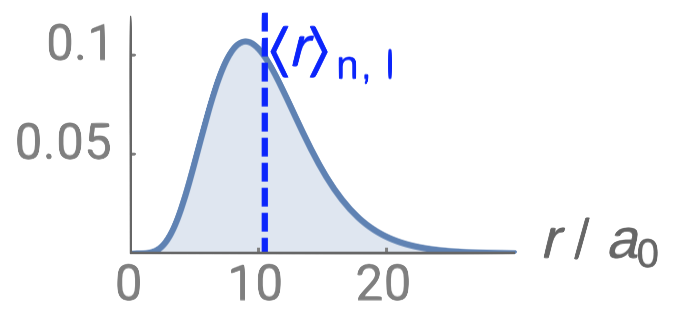0		2		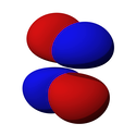2