3.3: Associative Mechanism and Kinetics
- Page ID
- 189848
\( \newcommand{\vecs}[1]{\overset { \scriptstyle \rightharpoonup} {\mathbf{#1}} } \)
\( \newcommand{\vecd}[1]{\overset{-\!-\!\rightharpoonup}{\vphantom{a}\smash {#1}}} \)
\( \newcommand{\dsum}{\displaystyle\sum\limits} \)
\( \newcommand{\dint}{\displaystyle\int\limits} \)
\( \newcommand{\dlim}{\displaystyle\lim\limits} \)
\( \newcommand{\id}{\mathrm{id}}\) \( \newcommand{\Span}{\mathrm{span}}\)
( \newcommand{\kernel}{\mathrm{null}\,}\) \( \newcommand{\range}{\mathrm{range}\,}\)
\( \newcommand{\RealPart}{\mathrm{Re}}\) \( \newcommand{\ImaginaryPart}{\mathrm{Im}}\)
\( \newcommand{\Argument}{\mathrm{Arg}}\) \( \newcommand{\norm}[1]{\| #1 \|}\)
\( \newcommand{\inner}[2]{\langle #1, #2 \rangle}\)
\( \newcommand{\Span}{\mathrm{span}}\)
\( \newcommand{\id}{\mathrm{id}}\)
\( \newcommand{\Span}{\mathrm{span}}\)
\( \newcommand{\kernel}{\mathrm{null}\,}\)
\( \newcommand{\range}{\mathrm{range}\,}\)
\( \newcommand{\RealPart}{\mathrm{Re}}\)
\( \newcommand{\ImaginaryPart}{\mathrm{Im}}\)
\( \newcommand{\Argument}{\mathrm{Arg}}\)
\( \newcommand{\norm}[1]{\| #1 \|}\)
\( \newcommand{\inner}[2]{\langle #1, #2 \rangle}\)
\( \newcommand{\Span}{\mathrm{span}}\) \( \newcommand{\AA}{\unicode[.8,0]{x212B}}\)
\( \newcommand{\vectorA}[1]{\vec{#1}} % arrow\)
\( \newcommand{\vectorAt}[1]{\vec{\text{#1}}} % arrow\)
\( \newcommand{\vectorB}[1]{\overset { \scriptstyle \rightharpoonup} {\mathbf{#1}} } \)
\( \newcommand{\vectorC}[1]{\textbf{#1}} \)
\( \newcommand{\vectorD}[1]{\overrightarrow{#1}} \)
\( \newcommand{\vectorDt}[1]{\overrightarrow{\text{#1}}} \)
\( \newcommand{\vectE}[1]{\overset{-\!-\!\rightharpoonup}{\vphantom{a}\smash{\mathbf {#1}}}} \)
\( \newcommand{\vecs}[1]{\overset { \scriptstyle \rightharpoonup} {\mathbf{#1}} } \)
\(\newcommand{\longvect}{\overrightarrow}\)
\( \newcommand{\vecd}[1]{\overset{-\!-\!\rightharpoonup}{\vphantom{a}\smash {#1}}} \)
\(\newcommand{\avec}{\mathbf a}\) \(\newcommand{\bvec}{\mathbf b}\) \(\newcommand{\cvec}{\mathbf c}\) \(\newcommand{\dvec}{\mathbf d}\) \(\newcommand{\dtil}{\widetilde{\mathbf d}}\) \(\newcommand{\evec}{\mathbf e}\) \(\newcommand{\fvec}{\mathbf f}\) \(\newcommand{\nvec}{\mathbf n}\) \(\newcommand{\pvec}{\mathbf p}\) \(\newcommand{\qvec}{\mathbf q}\) \(\newcommand{\svec}{\mathbf s}\) \(\newcommand{\tvec}{\mathbf t}\) \(\newcommand{\uvec}{\mathbf u}\) \(\newcommand{\vvec}{\mathbf v}\) \(\newcommand{\wvec}{\mathbf w}\) \(\newcommand{\xvec}{\mathbf x}\) \(\newcommand{\yvec}{\mathbf y}\) \(\newcommand{\zvec}{\mathbf z}\) \(\newcommand{\rvec}{\mathbf r}\) \(\newcommand{\mvec}{\mathbf m}\) \(\newcommand{\zerovec}{\mathbf 0}\) \(\newcommand{\onevec}{\mathbf 1}\) \(\newcommand{\real}{\mathbb R}\) \(\newcommand{\twovec}[2]{\left[\begin{array}{r}#1 \\ #2 \end{array}\right]}\) \(\newcommand{\ctwovec}[2]{\left[\begin{array}{c}#1 \\ #2 \end{array}\right]}\) \(\newcommand{\threevec}[3]{\left[\begin{array}{r}#1 \\ #2 \\ #3 \end{array}\right]}\) \(\newcommand{\cthreevec}[3]{\left[\begin{array}{c}#1 \\ #2 \\ #3 \end{array}\right]}\) \(\newcommand{\fourvec}[4]{\left[\begin{array}{r}#1 \\ #2 \\ #3 \\ #4 \end{array}\right]}\) \(\newcommand{\cfourvec}[4]{\left[\begin{array}{c}#1 \\ #2 \\ #3 \\ #4 \end{array}\right]}\) \(\newcommand{\fivevec}[5]{\left[\begin{array}{r}#1 \\ #2 \\ #3 \\ #4 \\ #5 \\ \end{array}\right]}\) \(\newcommand{\cfivevec}[5]{\left[\begin{array}{c}#1 \\ #2 \\ #3 \\ #4 \\ #5 \\ \end{array}\right]}\) \(\newcommand{\mattwo}[4]{\left[\begin{array}{rr}#1 \amp #2 \\ #3 \amp #4 \\ \end{array}\right]}\) \(\newcommand{\laspan}[1]{\text{Span}\{#1\}}\) \(\newcommand{\bcal}{\cal B}\) \(\newcommand{\ccal}{\cal C}\) \(\newcommand{\scal}{\cal S}\) \(\newcommand{\wcal}{\cal W}\) \(\newcommand{\ecal}{\cal E}\) \(\newcommand{\coords}[2]{\left\{#1\right\}_{#2}}\) \(\newcommand{\gray}[1]{\color{gray}{#1}}\) \(\newcommand{\lgray}[1]{\color{lightgray}{#1}}\) \(\newcommand{\rank}{\operatorname{rank}}\) \(\newcommand{\row}{\text{Row}}\) \(\newcommand{\col}{\text{Col}}\) \(\renewcommand{\row}{\text{Row}}\) \(\newcommand{\nul}{\text{Nul}}\) \(\newcommand{\var}{\text{Var}}\) \(\newcommand{\corr}{\text{corr}}\) \(\newcommand{\len}[1]{\left|#1\right|}\) \(\newcommand{\bbar}{\overline{\bvec}}\) \(\newcommand{\bhat}{\widehat{\bvec}}\) \(\newcommand{\bperp}{\bvec^\perp}\) \(\newcommand{\xhat}{\widehat{\xvec}}\) \(\newcommand{\vhat}{\widehat{\vvec}}\) \(\newcommand{\uhat}{\widehat{\uvec}}\) \(\newcommand{\what}{\widehat{\wvec}}\) \(\newcommand{\Sighat}{\widehat{\Sigma}}\) \(\newcommand{\lt}{<}\) \(\newcommand{\gt}{>}\) \(\newcommand{\amp}{&}\) \(\definecolor{fillinmathshade}{gray}{0.9}\)We can measure the rate of an associative reaction and make changes in the reaction conditions to see how the rate is affected. For example, we could easily change the concentrations of the two reactants. All we have to do is change the amount of reactant we dissolve in the solution.
If we did that, we would find a linear relationship between each concentration and rate. If we double the concentration of new ligand, the rate of reaction doubles. If we triple it, the rate triples.
Also, if we double the amount of metal complex, the rate doubles and so on.
We can write the following expression, called the rate law, to describe this relationship:
Rate Law: \(Rate = \frac{-d[ML_{n}]}{dt} = k[ML_{n}][L^{'}]\)
This type of reaction is sometimes called a second order reaction. That term just refers to the mathematical form of the rate law, which depends on concentration times concentration, or concentration squared. The "order" of the reaction is the number of concentrations multiplied together in the rate law.
Why does the associative mechanism depend on concentrations in this specific way?
This is a case of two molecules coming together. If both compounds are dissolved in solution, they must “swim around” or travel through the solution until they bump into each other and react. The more concentrated the solution is, or the more crowded it is with molecules, the more likely are the reactants to bump into each other. If we double the amount of new ligand in solution, an encounter between ligand and complex becomes twice as likely. If we double the amount of metal complex in solution, an encounter also becomes twice as likely.
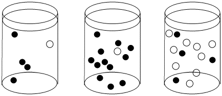
Figure \(\PageIndex{1}\): The effect of concentration on collision probability. In the first beaker, there is a chance that a black molecule and white molecule will meet and react together. The chance of a meeting is much higher in both the second beaker, where there are lots more black molecules, and in the third beaker, where there are many more white molecules.
Given the associative rate law above, what would happen to the reaction rate for an associative substitution in the following cases?
- the concentration of ligand is doubled, and the concentration of metal complex is doubled
- the concentration of ligand is tripled, and the concentration of metal complex is doubled
- the concentration of ligand is tripled, and the concentration of metal complex is tripled
- the concentration of ligand is halved, and the concentration of metal complex is doubled
- Answer a
-
Associative Rate Law: \(Rate = [ML_{n}][X]\), if MLn is the complex and X is the new ligand.
Rate will quadruple: \(Rate = (2 \times [ML_{n}]_{0}) \times (2 \times [X]_{0})= 4 \times [ML_{n}]_{0}[X]_{0}\), if [X]0 and [MLn]0 are the original concentrations.
- Answer b
-
Rate will sextuple: \(Rate = (3 \times [ML_{n}]_{0}) \times (2 \times [X]_{0}) = 6 \times [ML_{n}]_{0}[X]_{0}\).
- Answer c
-
Rate will nonuple: \(Rate = (3 \times [ML_{n}]_{0}) \times (3 \times [X]_{0}) = 9 \times [ML_{n}]_{0}[X]_{0}\).
- Answer d
-
Rate will stay the same: \(Rate = (0.5 \times [ML_{n}]_{0}) \times (2 \times [X]_{0}) = 1 \times [ML_{n}]_{0}[X]_{0}\).
Plot graphs of initial rate vs. concentration to show what you would see in associative substitution.
a) The concentration of new ligand, [X], is held constant at 0.1 mol/L and the concentration of metal complex is changed from 0.5 mol/L to 1 mol/L and then to 1.5 mol/L.
b) The concentration of metal complex, [MLn], is held constant at 0.1 mol/L and the concentration of ligand is changed from 0.5 mol/L to 1 mol/L and then to 1.5 mol/L.
- Answer
-
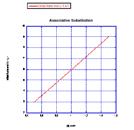
In the previous problem, the experiment was run in a particular way for particular reasons.
a) Why was one concentration held constant while the other one was changed? Why not change both?
b) Why does the graph report "initial rate" -- just the rate at the very beginning of the reaction?
- Answer a
-
Changing both concentrations at once would leave some doubt about whether one concentration had affected the rate, or the other concentration, or both. In practice, one concentration is usually held constant while the other is kept in excess and varied.
- Answer b
-
Rate changes over time because the concentrations of reactants change as they are consumed. By reporting only the initial rate (usually meaning less than 5% or 10% complete, but possibly even less than that if a lot of data can be gathered very quickly), the concentrations are still about what you started with. That means you can report a rate that corresponds to a given concentration with confidence.
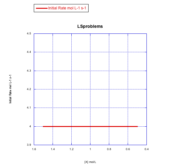
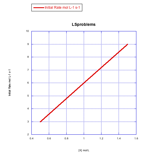
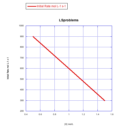
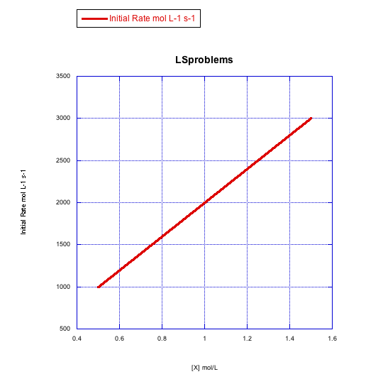
Given the following sets of initial rate data (rates measured at the beginning of a reaction), determine whether each case represents an associative substitution.
a)
b)
c)
d)
Answer a-
The rate would change with the ligand concentration if associative. This rate is constant over a range of ligand concentrations, so the reaction is not associative.
- Answer b
-
The rate increases linearly with ligand concentration. This reaction proceeds via an associative mechanism.
- Answer c
-
The rate changes over the concentration range, but it decreases. This is the opposite of what should happen. This reaction does not follow a simple associative pathway.
- Answer d
-
The rate increases linearly with ligand concentration. This reaction proceeds via an associative mechanism.
What information can be gained from the slopes of lines in Exercise \(\PageIndex{4}\) (Problem LS3.4.)?
- Answer
-
Because \(Rate = k[ML_{n}][L]\) is held constant while [L] is varied, then the slope of the line is k [MLn]. Since you would know the value of [MLn], you could obtain the rate constant from the quantity (slope/ [MLn]).


