
2.6: Characterization- The Mathematics Behind Enzyme Kinetics
- Page ID
- 189844

\( \newcommand{\vecs}[1]{\overset { \scriptstyle \rightharpoonup} {\mathbf{#1}} } \)
\( \newcommand{\vecd}[1]{\overset{-\!-\!\rightharpoonup}{\vphantom{a}\smash {#1}}} \)
\( \newcommand{\id}{\mathrm{id}}\) \( \newcommand{\Span}{\mathrm{span}}\)
( \newcommand{\kernel}{\mathrm{null}\,}\) \( \newcommand{\range}{\mathrm{range}\,}\)
\( \newcommand{\RealPart}{\mathrm{Re}}\) \( \newcommand{\ImaginaryPart}{\mathrm{Im}}\)
\( \newcommand{\Argument}{\mathrm{Arg}}\) \( \newcommand{\norm}[1]{\| #1 \|}\)
\( \newcommand{\inner}[2]{\langle #1, #2 \rangle}\)
\( \newcommand{\Span}{\mathrm{span}}\)
\( \newcommand{\id}{\mathrm{id}}\)
\( \newcommand{\Span}{\mathrm{span}}\)
\( \newcommand{\kernel}{\mathrm{null}\,}\)
\( \newcommand{\range}{\mathrm{range}\,}\)
\( \newcommand{\RealPart}{\mathrm{Re}}\)
\( \newcommand{\ImaginaryPart}{\mathrm{Im}}\)
\( \newcommand{\Argument}{\mathrm{Arg}}\)
\( \newcommand{\norm}[1]{\| #1 \|}\)
\( \newcommand{\inner}[2]{\langle #1, #2 \rangle}\)
\( \newcommand{\Span}{\mathrm{span}}\) \( \newcommand{\AA}{\unicode[.8,0]{x212B}}\)
\( \newcommand{\vectorA}[1]{\vec{#1}} % arrow\)
\( \newcommand{\vectorAt}[1]{\vec{\text{#1}}} % arrow\)
\( \newcommand{\vectorB}[1]{\overset { \scriptstyle \rightharpoonup} {\mathbf{#1}} } \)
\( \newcommand{\vectorC}[1]{\textbf{#1}} \)
\( \newcommand{\vectorD}[1]{\overrightarrow{#1}} \)
\( \newcommand{\vectorDt}[1]{\overrightarrow{\text{#1}}} \)
\( \newcommand{\vectE}[1]{\overset{-\!-\!\rightharpoonup}{\vphantom{a}\smash{\mathbf {#1}}}} \)
\( \newcommand{\vecs}[1]{\overset { \scriptstyle \rightharpoonup} {\mathbf{#1}} } \)
\( \newcommand{\vecd}[1]{\overset{-\!-\!\rightharpoonup}{\vphantom{a}\smash {#1}}} \)
\(\newcommand{\avec}{\mathbf a}\) \(\newcommand{\bvec}{\mathbf b}\) \(\newcommand{\cvec}{\mathbf c}\) \(\newcommand{\dvec}{\mathbf d}\) \(\newcommand{\dtil}{\widetilde{\mathbf d}}\) \(\newcommand{\evec}{\mathbf e}\) \(\newcommand{\fvec}{\mathbf f}\) \(\newcommand{\nvec}{\mathbf n}\) \(\newcommand{\pvec}{\mathbf p}\) \(\newcommand{\qvec}{\mathbf q}\) \(\newcommand{\svec}{\mathbf s}\) \(\newcommand{\tvec}{\mathbf t}\) \(\newcommand{\uvec}{\mathbf u}\) \(\newcommand{\vvec}{\mathbf v}\) \(\newcommand{\wvec}{\mathbf w}\) \(\newcommand{\xvec}{\mathbf x}\) \(\newcommand{\yvec}{\mathbf y}\) \(\newcommand{\zvec}{\mathbf z}\) \(\newcommand{\rvec}{\mathbf r}\) \(\newcommand{\mvec}{\mathbf m}\) \(\newcommand{\zerovec}{\mathbf 0}\) \(\newcommand{\onevec}{\mathbf 1}\) \(\newcommand{\real}{\mathbb R}\) \(\newcommand{\twovec}[2]{\left[\begin{array}{r}#1 \\ #2 \end{array}\right]}\) \(\newcommand{\ctwovec}[2]{\left[\begin{array}{c}#1 \\ #2 \end{array}\right]}\) \(\newcommand{\threevec}[3]{\left[\begin{array}{r}#1 \\ #2 \\ #3 \end{array}\right]}\) \(\newcommand{\cthreevec}[3]{\left[\begin{array}{c}#1 \\ #2 \\ #3 \end{array}\right]}\) \(\newcommand{\fourvec}[4]{\left[\begin{array}{r}#1 \\ #2 \\ #3 \\ #4 \end{array}\right]}\) \(\newcommand{\cfourvec}[4]{\left[\begin{array}{c}#1 \\ #2 \\ #3 \\ #4 \end{array}\right]}\) \(\newcommand{\fivevec}[5]{\left[\begin{array}{r}#1 \\ #2 \\ #3 \\ #4 \\ #5 \\ \end{array}\right]}\) \(\newcommand{\cfivevec}[5]{\left[\begin{array}{c}#1 \\ #2 \\ #3 \\ #4 \\ #5 \\ \end{array}\right]}\) \(\newcommand{\mattwo}[4]{\left[\begin{array}{rr}#1 \amp #2 \\ #3 \amp #4 \\ \end{array}\right]}\) \(\newcommand{\laspan}[1]{\text{Span}\{#1\}}\) \(\newcommand{\bcal}{\cal B}\) \(\newcommand{\ccal}{\cal C}\) \(\newcommand{\scal}{\cal S}\) \(\newcommand{\wcal}{\cal W}\) \(\newcommand{\ecal}{\cal E}\) \(\newcommand{\coords}[2]{\left\{#1\right\}_{#2}}\) \(\newcommand{\gray}[1]{\color{gray}{#1}}\) \(\newcommand{\lgray}[1]{\color{lightgray}{#1}}\) \(\newcommand{\rank}{\operatorname{rank}}\) \(\newcommand{\row}{\text{Row}}\) \(\newcommand{\col}{\text{Col}}\) \(\renewcommand{\row}{\text{Row}}\) \(\newcommand{\nul}{\text{Nul}}\) \(\newcommand{\var}{\text{Var}}\) \(\newcommand{\corr}{\text{corr}}\) \(\newcommand{\len}[1]{\left|#1\right|}\) \(\newcommand{\bbar}{\overline{\bvec}}\) \(\newcommand{\bhat}{\widehat{\bvec}}\) \(\newcommand{\bperp}{\bvec^\perp}\) \(\newcommand{\xhat}{\widehat{\xvec}}\) \(\newcommand{\vhat}{\widehat{\vvec}}\) \(\newcommand{\uhat}{\widehat{\uvec}}\) \(\newcommand{\what}{\widehat{\wvec}}\) \(\newcommand{\Sighat}{\widehat{\Sigma}}\) \(\newcommand{\lt}{<}\) \(\newcommand{\gt}{>}\) \(\newcommand{\amp}{&}\) \(\definecolor{fillinmathshade}{gray}{0.9}\)Michaelis-Menten Plots
An enzyme-catalysed reaction can be roughly divided into three stages: enzyme-substrate binding, "catalysis" and product release. "Catalysis" refers to all the steps that happen to convert substrate into product. Sometimes, these steps are too fast to distinguish from each other. To simplify, we sometimes refer to this whole sequence of events as though they were just one step.
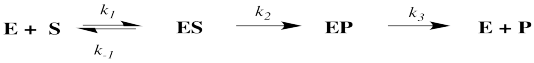
Often, but not always, that catalysis part is the rate determining step. Product release is sort of an afterthought.
In that case, we might simplify and only consider those steps up through catalysis.
If we do that, we find that enzyme reactions can be summarized by a relation called the Michaelis-Menten equation, named after the early 20th century biochemist Leonor Michaels and his collaborator, the immensely talented artist, physician and biochemist, Maud Menten.
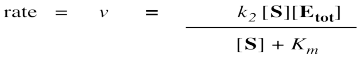
The numerator in this equation should make sense -- of course the rate should increase when we add either more substrate or more enzyme and the relationship will depend on the speed of that product-forming step.
The denominator is a little more complicated and contains the composite constant Km, the Michaelis-Menten constant.
This relationship can be understood most easily by examining its limits. For instance, suppose the substrate concentration is still very low. Perhaps it is much smaller than Km. How does that affect the rate of the reaction?
It is useful to keep in mind that a large number added to a small number is just a large number. One million plus one is about a million. One million plus three is also about a million. One million plus five is pretty close to a million. We can often ignore the small quantity in additions. In that sense, if [S] is small, we can ignore it in the denominator, and think of the denominator instead as "approximately Km".
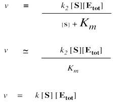
We can't ignore [S] in the numerator, of course, even if it is very small. That's because a number multiplied by a very small number also becomes a very small number; the small number really counts when it is multiplied by something.
On the other hand, when [S] gets very large, we can ignore Km. That means Km disappears from the denominator, leaving only [S]. At that point, the [S] in the denominator and numerator cancels.
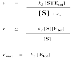
Remember, when [S] gets very large, the reaction has reached its maximum possible rate, because the enzyme is saturated. Adding more substrate doesn't speed things up, because the extra substrate just has to wait around until an enzyme becomes available. We call that maximum rate Vmax.
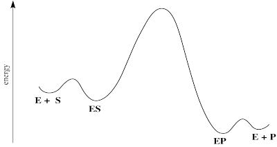
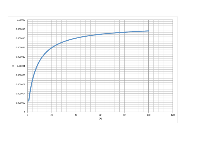
- The limits of the Michaelis Menten equation explains the shape of the curve describing the rate dependence on substrate.
There is another piece of useful information we can get from this equation. It comes at an intermediate point between the two cases we have considered so far. What if the numerical value of Km and [S] are exactly equal? In that case, the value of the denominator, Km + [S], is the same as [S] + [S]. The denominator becomes 2[S]. Just as in the limiting case that gave us the value of Vmax, the [S] cancels, but this time there is still a 2 in the denominator, so we get Vmax/2.
Turning that conclusion around, if we find the point on a Michaelis Menten plot where the rate is half the maximum rate, we can drop a line down to the x axis. The value of [S] at the intercept will be numerically the same as the value of Km.
- Vmax is the point on the y axis where the rate has completely leveled off.
- Km is the point on the x axis corresponding to y = Vmax/2.
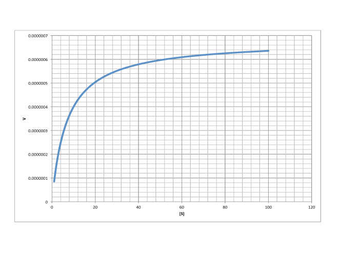
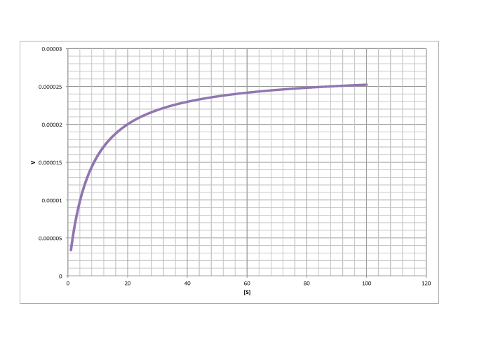
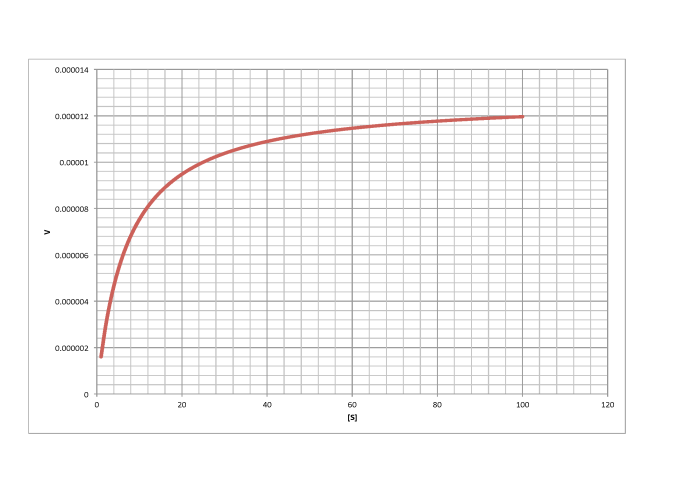
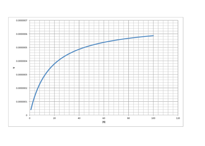
Determine Vmax and Km in each of the following cases. Assume the units of [S] are millimoles per liter and the units of V are moles per liter per second.
a)
b)
c)
d)
e)
Answer a-
\[V_{max} = 1.8 \times 10^{-5} \frac{mol}{L s} \nonumber\]
\[\frac{V_{max}}{2} = 9 \times 10^{-6} \frac{mol}{L s}\) so \(K_{m} = 6 \frac{mol}{L} \nonumber\]
- Answer b
-
\[V_{max} = 6.5 \times 10^{-7} \frac{mol}{L s} \nonumber\]
\[\frac{V_{max}}{2} = 3.25 \times 10^{-7} \frac{mol}{L s}\) so \(K_{m} = 7 \frac{mol}{L} \nonumber\]
- Answer c
-
\[V_{max} = 2.6 \times 10^{-5} \frac{mol}{L s} \nonumber\]
\[\frac{V_{max}}{2} = 1.3 \times 10^{-5} \frac {mol}{L s}\) so \(K_{m} = 6 \frac{mol}{L} \nonumber\]
- Answer d
-
\[V_{max} = 1.2 \times 10^{-5} \frac{mol}{L s} \nonumber\]
\[\frac{V_{max}}{2} = 6 \times 10^{-6} \frac{mol}{L s}\) so \(K_{m} = 6 \frac{mol}{L} \nonumber\]
- Answer e
-
\[V_{max} = 6.0 \times 10^{-7} \frac{mol}{L s} \nonumber\]
\[\frac{V_{max}}{2} = 3 \times 10^{-7} \frac {mol}{L s}\) so \(K_{m} = 13 \frac {mol}{L} \nonumber\]
Turnover Frequency and Efficiency
If we're running an experiment, we know what the total concentration of enzyme is, because we're the ones who put it in there. That means that we can also figure out exactly what that rate constant is for catalysis.
\[k_{cat} = k_{2} = \frac{V_{max}}{\mathbf{[E_{tot}]}} \nonumber\]
That quantity, kcat, is sometimes referred to by biochemists as the "turnover number". The turnover number essentially means the number of molecules of product made by an enzyme in the specified period of time (usually the units of kcat are expressed as s-1, but they could also be written in min-1, etc).
In industrial catalysis, kcat is instead referred to as the "turnover frequency", but of course it still means the same thing. There is an important reason for this difference in terms. The "turnover number" in industry refers to the number of molecules of product made before the catalyst stops working. Catalyst death can occur for any number of reasons, but you might imagine something going wrong via a side reaction that renders the catalyst unreactive toward the substrate. This is a very important consideration in industry. The engineer in charge of the production plant would like to replace the catalyst with a new batch before it stops working, to avoid an unscheduled halt in the process that could prove very costly. They need to have an idea about when that is likely to happen, so they need to be aware of the turnover number in this sense.
Another consideration that is sometimes useful is enzymatic efficiency. Remember, the reaction does not depend only on the catalysis step. The binding step also matters. The faster the catalysis step, the faster the production of product. In addition, the greater the proportion of substrate bound, the faster the production of product.
Combining those two ideas:
\[Efficiency = \frac{k_{cat}}{K_{m}} \nonumber\]
In this relationship, Km is a stand-in for the equilibrium constant for enzyme-substrate dissociation. It's not quite the same thing, but it's the closest we've got. By extension, 1/Km stands for the enzyme-substrate binding constant. The greater the binding constant and the faster the catalysis, the more efficient the enzyme.
Note that the units of Km are concentration units (mol L-1, for instance). The units of efficiency will therefore be something like L mol-1 s-1.
Lineweaver-Burk Plots
The Michaelis-Menten equation is useful in other ways, too. If we take its inverse, we get a new relationship.
That's useful because it's really an expression for a straight line. If we plot 1/v against 1/[S], we get a straight line. The slope is Km/Vmax and the y intercept is 1/Vmax.
- Lineweaver-Burk plot gives a straight line for the rate data.
- y intercept = 1/Vmax
- slope = Km/Vmax
- the x intercept = -1/Km, too
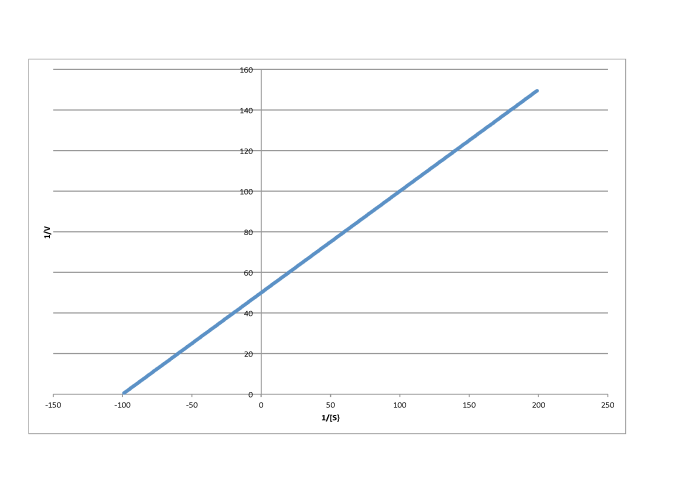
Determine the values of Vmax and Km in each of the following cases. Assume the units of [S] are millimoles per liter and the units of V are moles per liter per second.
a)
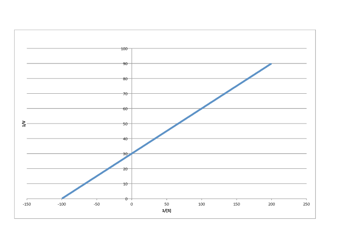
b)
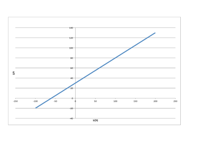
c)
d)
e)
f)
Answer a-
\[\frac{1}{V_{max}} = 30 \frac{ L s}{mol}\) so \(V_{max} = 3.3 \times 10^{-2} \frac {mol}{L s} \nonumber\]
\[\frac{-1}{K_{m} = -40 \frac{L}{mmol}\) so \(K_{m} = 2.5 \times 10^{-2} \frac{M}{L} \nonumber\]
- Answer b
-
\[\frac{1}{V_{max}} = 50 \frac{L s}{mol}\) so \(V_{max} = 2.- \times 10^{-2} \frac{mol}{L s} \nonumber\]
\(\frac{-1}{K_{m} = -70 \frac{L}{mmol}\) so \(K_{m} = 1.4 \times 10^{-2} \frac{M}{L}\)
- Answer c
-
\[\frac{1}{V_{max} = 60 \frac{L s}{mol}\) so \(V_{max} = 1.7 \times 10^{-2} \frac{mol}{L s} \nonumber\]
\(\frac{-1}{K_{m}} = -70 \frac{L}{mmol}\) so \( K_{m} = 1.4 \times 10^{-2} \frac{M}{L}\)
- Answer d
-
\[\frac{1}{V_{max}} = 50 \frac{L s}{mol}\) so \(V_{max} = 2.0 \times 10^{-2} \frac{mol}{L s} \nonumber\]
\(\frac{-1}{K_{m}} = -100 \frac {L}{mmol}\) so \(K_{m} = 1.0 \times 10^{-2} \frac{M}{L}\)
- Answer e
-
\[\frac{1}{V_{max}} = 30 \frac{L s}{mol}\) so \(V_{max} = 3.3 \times 10^{-2} \frac {mol}{L s} \nonumber\]
\(\frac{-1}{K_{m}} = -100 \frac{L}{mmol}\) so \(K_{m} = 1.0 \times 10^{-2} \frac{M}{L}\)
- Answer f
-
\[\frac{1}{V_{max}} = 30 \frac{L s}{mol}\) so \(V_{max} = 3.3 \times 10^{-2} \frac{mol}{L s} \nonumber\]
\(\frac{-1}{K_{m}} = -60 \frac{L}{mmol}\) so \(K_{m} = 1.7 \times 10^{-2} \frac{M}{L}\)
Inhibition and Lineweaver-Burk Plots
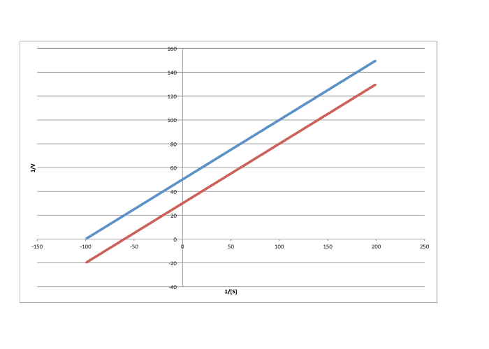
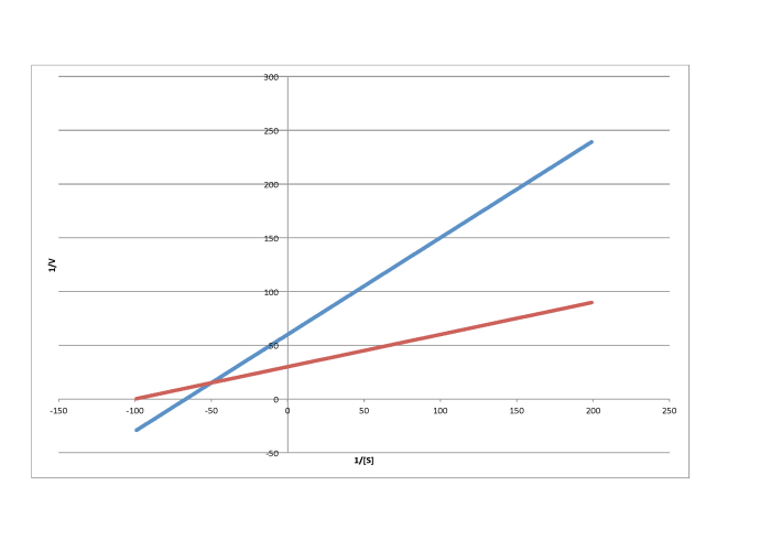
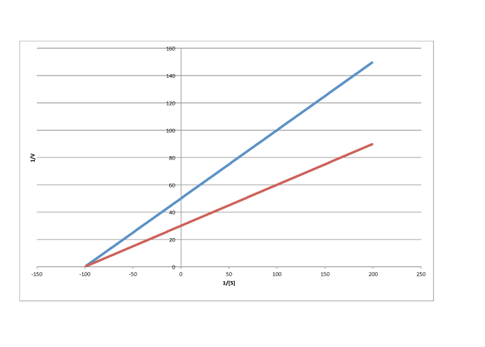
Lineweaver-Burk plots allow additional insight into the mechanism of inhibition. The following plot, for example, shows competitive inhibition.
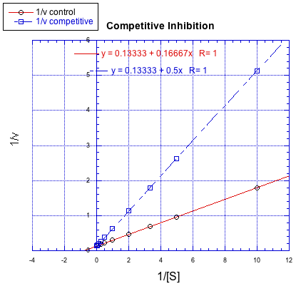
Because the plot uses 1/v on the y axis, the slower reaction is actually the top line. The bottom line is the regular reaction without an inhibitor. Remember, the y intercept is equal to 1/Vmax. In competitive inhibition, the inhibited reaction eventually reaches (or at least approaches) the same Vmax as the uninhibited reaction. The Lineweaver-Burk plot shows both lines meet the y axis at the same place.
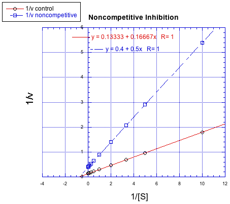
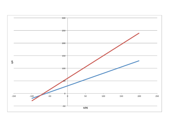
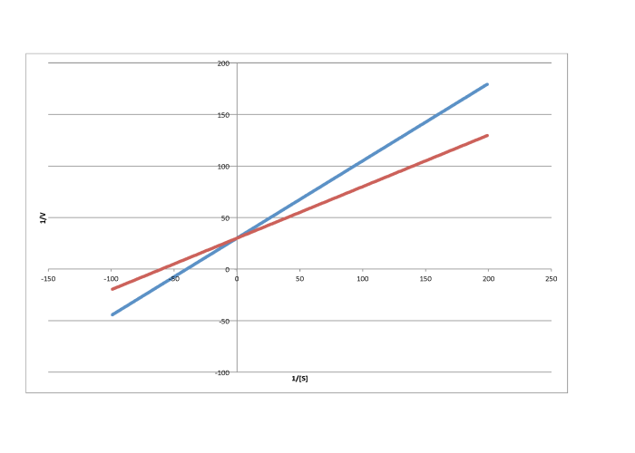
In contrast, the following plot shows noncompetitive inhibition. Once again, the regular line is the lower one, whereas the upper line is the inhibited one. The two lines do not share the same y intercept, however. However, they do share the same x intercept. That's because noncompetitive inhibition does not directly affect binding of substrate (which is reflected in Km), but interferes with the catalysis step (linked to Vmax).
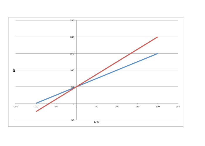
The difference between noncompetitive and uncompetitive inhibition, very subtle in a Michaelis-Menten plot, is quite clear in Lineweaver-Burk. The case illustrated below is thought of as "pure" uncompetitive inhibition. Once again, the inhibited reaction is shown by the upper line. In this case, the inhibited and uninhibited reactions produce parallel lines in the Lineweaver-Burk plot; that feature is actually the definition of uncompetitive inhibition.
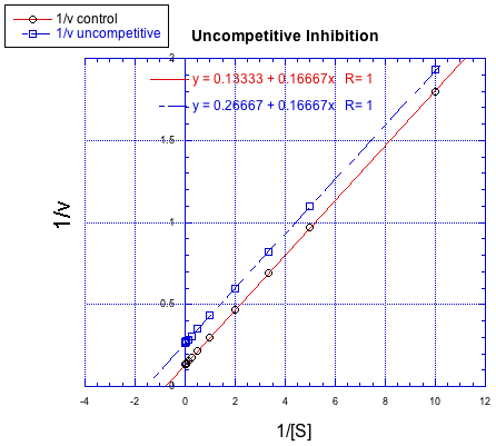
If you think about it, pure uncompetitive inhibition only happens under very specific circumstances. The Km clearly differs when an inhibitor is added; we can see that in the different x intercept. However, the slope is the same. The slope is Km/Vmax. That means that, because Km is different, Vmax must differ in exactly the same way, keeping the slope the same. For example, if Km is cut in half in the inhibited reaction, then Vmax must also be cut in half. That would keep the slope the same.
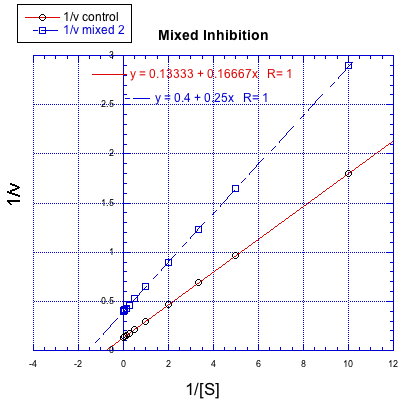
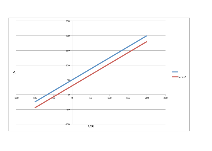
On the other hand, a situation in which the inhibited reaction does not give a line parallel to the regular reaction is called "mixed inhibition". Like uncompetitive inhibition, mixed inhibition results in changes in both Km and Vmax. However, the changes in this case do not scale exactly the same way as in uncompetitive inhibition.
Characterise each of the following graphs as representing competitive, noncompetitive, uncompetitive, or mixed inhibition.
a)
b)
c)
d)
e)
f)
g)
Answer a-
uncompetitive
- Answer b
-
mixed
- Answer c
-
noncompetitive
- Answer d
-
competitive
- Answer e
-
uncompetitive
- Answer f
-
noncompetitive
- Answer g
-
competitive
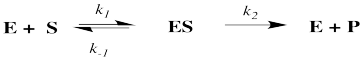
The Origin of the Michaelis-Menten Equation
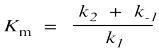
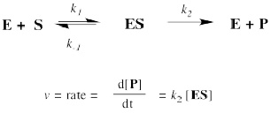
But where does the Michaelis-Menten relationship come from? That takes a little bit of heavy lifting with kinetics. If you feel the need to know, then we'll start with the approximation that the reaction essentially boils down to two steps: substrate binding and the stuff after that. The binding step is described as k1/k-1. The stuff after that is summed up in k2.
The rate of product formation really depends on the rate of the elementary step k2. That rate depends upon the amount of enzyme substrate complex and its rate of passage through the subsequent step.
The trouble is, the enzyme substrate complex is an intermediate. We don't know exactly how much of it we have. We might assume that, as a reactive intermediate, the complex doesn't have much of a lifetime. It gets used up pretty much as soon as it forms.
That assumption helps us to express the concentration of enzyme substrate complex in terms of other things we might know more about: the enzyme and the substrate. Of course, the enzyme and the substrate react together to make the enzyme substrate complex. They react together with rate constant k1.
Two possible fates await the enzyme substrate complex. Either it is released back to enzyme and free substrate, with rate constant k-1, or else it goes on to make product, with rate constant k2. In a steady state approximation, the enzyme substrate complex is consumed as soon as it is formed.
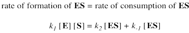
Again, we don't know how much free enzyme there is. We don't know how much enzyme-substrate complex we have. We do know how much enzyme is added at the beginning of the kinetics experiment. We'll call that concentration [Etot], meaning the total amount of enzyme. Some of that enzyme remains free, and some of it is bound as enzyme-substrate complex.
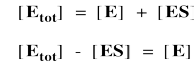
It's useful to express the concentration of free enzyme as the total enzyme minus that portion bound with substrate. That way, we'll be able to eliminate the term for free enzyme from the rate equation. A few steps of algebra let us express the concentration of the enzyme-substrate complex solely in terms of the total enzyme concentration, the substrate concentration and some rate constants.
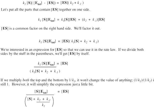
Remember, the rate of product formation just depends on the amount of enzyme-substrate complex and the rate constant for the catalysis step.
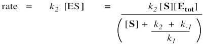
That collection of constants in the denominator is just a group of numbers. It's a constant. We'll call it the Michaelis-Menten constant.
That brings us back to the Michaelis-Menten equation.