
Atomic Orbitals
- Page ID
- 53284
\( \newcommand{\vecs}[1]{\overset { \scriptstyle \rightharpoonup} {\mathbf{#1}} } \)
\( \newcommand{\vecd}[1]{\overset{-\!-\!\rightharpoonup}{\vphantom{a}\smash {#1}}} \)
\( \newcommand{\dsum}{\displaystyle\sum\limits} \)
\( \newcommand{\dint}{\displaystyle\int\limits} \)
\( \newcommand{\dlim}{\displaystyle\lim\limits} \)
\( \newcommand{\id}{\mathrm{id}}\) \( \newcommand{\Span}{\mathrm{span}}\)
( \newcommand{\kernel}{\mathrm{null}\,}\) \( \newcommand{\range}{\mathrm{range}\,}\)
\( \newcommand{\RealPart}{\mathrm{Re}}\) \( \newcommand{\ImaginaryPart}{\mathrm{Im}}\)
\( \newcommand{\Argument}{\mathrm{Arg}}\) \( \newcommand{\norm}[1]{\| #1 \|}\)
\( \newcommand{\inner}[2]{\langle #1, #2 \rangle}\)
\( \newcommand{\Span}{\mathrm{span}}\)
\( \newcommand{\id}{\mathrm{id}}\)
\( \newcommand{\Span}{\mathrm{span}}\)
\( \newcommand{\kernel}{\mathrm{null}\,}\)
\( \newcommand{\range}{\mathrm{range}\,}\)
\( \newcommand{\RealPart}{\mathrm{Re}}\)
\( \newcommand{\ImaginaryPart}{\mathrm{Im}}\)
\( \newcommand{\Argument}{\mathrm{Arg}}\)
\( \newcommand{\norm}[1]{\| #1 \|}\)
\( \newcommand{\inner}[2]{\langle #1, #2 \rangle}\)
\( \newcommand{\Span}{\mathrm{span}}\) \( \newcommand{\AA}{\unicode[.8,0]{x212B}}\)
\( \newcommand{\vectorA}[1]{\vec{#1}} % arrow\)
\( \newcommand{\vectorAt}[1]{\vec{\text{#1}}} % arrow\)
\( \newcommand{\vectorB}[1]{\overset { \scriptstyle \rightharpoonup} {\mathbf{#1}} } \)
\( \newcommand{\vectorC}[1]{\textbf{#1}} \)
\( \newcommand{\vectorD}[1]{\overrightarrow{#1}} \)
\( \newcommand{\vectorDt}[1]{\overrightarrow{\text{#1}}} \)
\( \newcommand{\vectE}[1]{\overset{-\!-\!\rightharpoonup}{\vphantom{a}\smash{\mathbf {#1}}}} \)
\( \newcommand{\vecs}[1]{\overset { \scriptstyle \rightharpoonup} {\mathbf{#1}} } \)
\( \newcommand{\vecd}[1]{\overset{-\!-\!\rightharpoonup}{\vphantom{a}\smash {#1}}} \)
\(\newcommand{\avec}{\mathbf a}\) \(\newcommand{\bvec}{\mathbf b}\) \(\newcommand{\cvec}{\mathbf c}\) \(\newcommand{\dvec}{\mathbf d}\) \(\newcommand{\dtil}{\widetilde{\mathbf d}}\) \(\newcommand{\evec}{\mathbf e}\) \(\newcommand{\fvec}{\mathbf f}\) \(\newcommand{\nvec}{\mathbf n}\) \(\newcommand{\pvec}{\mathbf p}\) \(\newcommand{\qvec}{\mathbf q}\) \(\newcommand{\svec}{\mathbf s}\) \(\newcommand{\tvec}{\mathbf t}\) \(\newcommand{\uvec}{\mathbf u}\) \(\newcommand{\vvec}{\mathbf v}\) \(\newcommand{\wvec}{\mathbf w}\) \(\newcommand{\xvec}{\mathbf x}\) \(\newcommand{\yvec}{\mathbf y}\) \(\newcommand{\zvec}{\mathbf z}\) \(\newcommand{\rvec}{\mathbf r}\) \(\newcommand{\mvec}{\mathbf m}\) \(\newcommand{\zerovec}{\mathbf 0}\) \(\newcommand{\onevec}{\mathbf 1}\) \(\newcommand{\real}{\mathbb R}\) \(\newcommand{\twovec}[2]{\left[\begin{array}{r}#1 \\ #2 \end{array}\right]}\) \(\newcommand{\ctwovec}[2]{\left[\begin{array}{c}#1 \\ #2 \end{array}\right]}\) \(\newcommand{\threevec}[3]{\left[\begin{array}{r}#1 \\ #2 \\ #3 \end{array}\right]}\) \(\newcommand{\cthreevec}[3]{\left[\begin{array}{c}#1 \\ #2 \\ #3 \end{array}\right]}\) \(\newcommand{\fourvec}[4]{\left[\begin{array}{r}#1 \\ #2 \\ #3 \\ #4 \end{array}\right]}\) \(\newcommand{\cfourvec}[4]{\left[\begin{array}{c}#1 \\ #2 \\ #3 \\ #4 \end{array}\right]}\) \(\newcommand{\fivevec}[5]{\left[\begin{array}{r}#1 \\ #2 \\ #3 \\ #4 \\ #5 \\ \end{array}\right]}\) \(\newcommand{\cfivevec}[5]{\left[\begin{array}{c}#1 \\ #2 \\ #3 \\ #4 \\ #5 \\ \end{array}\right]}\) \(\newcommand{\mattwo}[4]{\left[\begin{array}{rr}#1 \amp #2 \\ #3 \amp #4 \\ \end{array}\right]}\) \(\newcommand{\laspan}[1]{\text{Span}\{#1\}}\) \(\newcommand{\bcal}{\cal B}\) \(\newcommand{\ccal}{\cal C}\) \(\newcommand{\scal}{\cal S}\) \(\newcommand{\wcal}{\cal W}\) \(\newcommand{\ecal}{\cal E}\) \(\newcommand{\coords}[2]{\left\{#1\right\}_{#2}}\) \(\newcommand{\gray}[1]{\color{gray}{#1}}\) \(\newcommand{\lgray}[1]{\color{lightgray}{#1}}\) \(\newcommand{\rank}{\operatorname{rank}}\) \(\newcommand{\row}{\text{Row}}\) \(\newcommand{\col}{\text{Col}}\) \(\renewcommand{\row}{\text{Row}}\) \(\newcommand{\nul}{\text{Nul}}\) \(\newcommand{\var}{\text{Var}}\) \(\newcommand{\corr}{\text{corr}}\) \(\newcommand{\len}[1]{\left|#1\right|}\) \(\newcommand{\bbar}{\overline{\bvec}}\) \(\newcommand{\bhat}{\widehat{\bvec}}\) \(\newcommand{\bperp}{\bvec^\perp}\) \(\newcommand{\xhat}{\widehat{\xvec}}\) \(\newcommand{\vhat}{\widehat{\vvec}}\) \(\newcommand{\uhat}{\widehat{\uvec}}\) \(\newcommand{\what}{\widehat{\wvec}}\) \(\newcommand{\Sighat}{\widehat{\Sigma}}\) \(\newcommand{\lt}{<}\) \(\newcommand{\gt}{>}\) \(\newcommand{\amp}{&}\) \(\definecolor{fillinmathshade}{gray}{0.9}\)Skills to Develop
- Illustrate the general shape of atomic orbitals
- Identify the relationship between quantum numbers
The "old quantum mechanics" introduced the idea of quantization, and it was good for describing the position of spectroscopic lines of single electron atoms. But it couldn't predict how strong the lines were. The "new quantum mechanics" of Schrodinger and Heisenberg took the wave-particle duality to its logical conclusion. While Bohr's model was still "classical" in that there was a defined orbit or trajectory (a path that could be calculated) for the electron, Schrodinger and Heisenberg changed that. Basically, where is a wave? If a particle behaves as a wave, you can't point to the exact spot where it is. Also, if light energy is quantized, it turns out that you can't measure the path taken by an electron without changing the path. In microscopy, which is using microscopes to look at small things, you can't separate things that are closer together than the wavelength used. This is why we use X-ray diffraction and electron microscopes with very short wavelengths to look at atoms and molecules. So if you want to measure the electron's path with light, and measure it precisely on an atomic scale, you have to use a short wavelength of light. But if you use a short wavelength then it has a lot of energy (E = hν), enough to change the electron's direction. This is the basis of the Uncertainty Principle.
The result of this (and also of Schrodinger's 3-D, space-filling wavefunction) is that we no longer describe electrons using orbits, or defined paths. Instead we talk about orbitals, which are defined by wavefunctions Ψ(x,y,z) like the one calculated in the previous section. It turns out (although I think Schrodinger didn't exactly intend this at first) that Ψ(x,y,z)2 is the probability of finding the "particle" at position (x,y,z).
Schrodinger found the standing waves or Ψ(x,y,z) for the electron in a hydrogen atom. These are much more complicated that the wavefunction we found because they are in 3-D and also have a potential energy to worry about. (But they aren't that complicated: you can look at them here.) There are an infinite number of functions that solve the equation, just like in the simple example. In the 1-D example, we used 1 quantum number n to determine the energies. As n increased, so did the energy, and so did the number of nodes (places where the amplitude is zero). In 3-D, the standing waves are specified by 3 quantum numbers. (Actually, Bohr and others were using 3 quantum numbers before Schrodinger published this, because it makes sense in 3-D.) The principal quantum number n corresponds roughly to the radius of the orbit in the Bohr model, or to the "most probable distance from the nucleus" in the orbital model. This also corresponds to the energy: the electron is lower energy when it is close to the nucleus, because of the Coulomb attraction. The second quantum number ℓ gives the shape. In the Bohr model this meant ellipse or circle. In Schrodinger's model the shapes are 3-D. You can look at them in detail on Wikipedia (scroll down to the table of images) or with an animated applet like this. This is also a good time to check out the "orbitals" tab on Ptable. Pick an element, then move over the arrows to see a picture of each orbital.
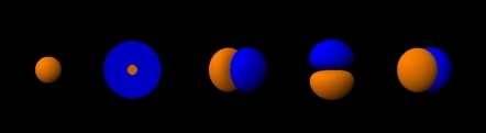
Finally, the third quantum number tells the orientation. In the Bohr model this meant what plane the orbit was in. In the figure, you can see that the last 3 orbitals have the same shape but point along different directions (x, y and z).
Notice that standard pictures of orbitals show most of them with 2 colors. This represents the phase of the orbital (whether Ψ is + or − at that point). This doesn't effect the energy or the probability of finding the particle there, but it is very important when atoms interact with each other, like forming bonds, which is what chemistry is all about! When waves interact with each other, it matters a lot whether the peak (high point) overlaps with the trough (low point) or not. This is true of water waves, sound waves, light waves and electron waves.
There are lots of ways of showing orbitals, but usually they just draw a surface so that you have 50% or 90% or whatever chance of finding the electron inside the surface. (Always, the probability of finding the electron becomes 0 as you get far enough from the nucleus.) The second orbital in the picture is shown as a slice, so you can see that the inside near the nucleus has the opposite phase as the outside. Wherever the color changes, there must be a node (Ψ passes through 0 as it goes from + or −). Thus the first orbital has no node, which makes sense because more nodes mean higher energy. The second has 1 spherical node. The next three have a planar (flat) node. If you look at more orbitals, you'll notice that the nodes keep increasing.
Here's the pattern of orbital shapes and quantum numbers.
- The principal quantum number n tells you how big the orbital is and what the energy is. It also tells you how many spherical nodes the orbital has. The values go from n = 1, 2, 3, 4, 5, 6, 7... they could keep going but we haven't found elements that need that many orbitals yet! The number of spherical nodes in the orbital is n − ℓ − 1.
- The angular momentum quantum number ℓ tells you the shape. If ℓ = 0, the orbital has spherical symmetry (it's round), and we say it is an "s orbital". If ℓ = 1, the orbital has one planar node, and it's called a "p orbital". See the figure below for d and f orbitals, with 2 and 3 planar nodes each. The possible values of ℓ are 0, 1, ... n − 1.
- The magnetic quantum number mℓ tells the orientation of the orbital. The possible values are -ℓ, -ℓ + 1, ... 0, 1, ℓ − 1, ℓ. For instance, for the p orbitals, it can be -1, 0, 1. You can remember the number of orientations using the table below.


A geometric pattern for remembering the number of each type of orbitals and the possible values of the quantum numbers.
Outside Links
- Atomic Orbitals Explained, by DCaulf (15 min)
Contributors and Attributions
Emily V Eames (City College of San Francisco)