4.7: Modelling exposure

3.8. Modelling exposure

3.8.1. How to estimate emission?

In preparation

3.8.2. Multicompartment modeling

Authors: Dik van de Meent and Michael Matthies

Reviewer: John Parsons

Learning objectives:

You should be able to

• explain what a mass balance equation is
• describe how mass balance equations are used in multimedia fate modeling
• explain the concepts of thermodynamic equilibrium and steady state

• give some examples of the use of multimedia mass balance modeling

Keywords: mass balance equation, environmental fate model

The mass balance equation

Multicompartment (or multimedia) mass balance modeling starts from the universal conservation principle, formulated as balance equation. The governing principle is that the rate of change (of any entity, in any system) equals the difference between the sum of all inputs (of that entity) to the system and the sum of all outputs from it. Environmental modelers use the balance equation to predict exposure concentrations of chemicals in the environment by deduction from knowledge of the rates of input- and output processes, which can be understood easiest from considering the mass balance equation for one single environmental compartment (Figure 1):

(eq. 1)

where dm^i,j/dt represents the change of mass of chemical i in compartment j (kg) over time (s), and input^i,j and output^i,j denote the rates of input and output of chemical to and from compartment j, respectively.

Figure 1. The mass of a chemical in a lake is like the mass of water in a leaking bucket: both can be described with the universal (mass) balance equation, which says differences in inputs and outputs make amounts held up in systems change: .

One compartment model

In multimedia mass balance modeling, mass balance equations (of the type shown in equation 1) are formulated for each environmental compartment. Outflows of chemical from the compartments are often proportional to the amounts of chemical present in the compartments, while external inputs (emissions) may often be assumed constant. In such cases, i.e. when first-order kinetics apply (see section 3.3 on Environmental fate of chemicals), mass balance equations take the form of equation 1 in section 3.3. For one compartment (e.g. a lake, as in Figure 1) only:

(eq. 2)

in which dm/dt (kg.s^-1) is the rate of change of the mass (kg) of chemical in the lake, I (kg.s^-1) is the (constant) emission rate, and the product k.m (kg.s^-1) denotes the first-order loss rate of the chemical from the lake. It is obvious that eventually a steady state must develop, in which the mass of chemical in the lake reaches a predictable maximum

(eq. 2a)

Figure 2):

Figure 2. For one compartment only, in case loss processes obey first-order kinetics and emissions are constant (i.e. not varying with time), the mass of chemical is expected to increase exponentially from its initial mass m₀ to its steady-state level , which will be reached at ininite time . After Van de Meent et al. (2011).

(eq. 3)

When the input rate (emission) is constant, i.e. that it does not vary with time, and is independent of the mass of chemical present, the mass of chemical in the systems is expected to increase exponentially, from its initial value at, to a steady level at . According to equation 3, a final mass level equal to is to be expected.

Multi-compartment model

The prefix 'multi' indicates that generally (many) more than one environmental compartment is considered. The Unit World (see below) contains air, water, biota, sediment and soil; more advanced global modeling systems may use hundreds of compartments. The case of three compartments (typically one air, one water, one soil) is schematically worked out in Figure 3.

Figure 3. Three-compartment mass balance model. Arrows represent mass flows of chemical to and from compartments. Losses from source compartments (negative signs) become gains to receiving compartments (positive sign). The model consists of three differential mass balance equations, with (nine) known rate constants k_i,j (for flows out of source compartments i, into receiving compartments j, in s^-1), and (three) unknown masses m_i (kg). From Van de Meent et al. (2011), with permission.

Each compartment can receive constant inputs (emissions, imports), and chemical can be exported from each compartment by degradation or advective outflow, as in the one-compartment model. In addition, chemical can be transported between compartments (simultaneous import-export). All mass flows are characterized by (pseudo) first-order rate constants (see section 3.3 on Environmental fate processes). The three mass balance equations eventually balance to zero at infinite time:

(eq. 4)

where the symbols denote mass in compartments i at steady state. Sets of n linear equations with n unknowns can be solved algebraically, by manually manipulating equations 4, until clean expressions for each of the three m_i values are obtained, which inevitably becomes tedious as soon as more than two mass balance equations are to be solved - this did not withhold one of Prof. Mackay's most famous PhD students from successfully solving a set of 14 equations! An easier way of solving sets of n linear equations with n unknowns is by means of linear algebra. Using linear algebraic vector-matrix calculus, the equations 4 can be rewritten into one linear-algebraic equation:

(eq. 5)

in which in which is the vector of masses in the three compartments, is the model matrix of known rate constants and is the vector of known emission rates:

The solution of equation 5 is

in which is the vector of masses at steady state and is the inverse of model matrix . The linear algebraic method of solving linear mass balance equations is easily carried with spreadsheet software (such as MS Excel, LibreOffice Calc or Google Sheets), which contain built-in array functions for inverting matrices and multiplying them by vectors.

Unit World modeling

In the late 1970s, pioneering environmental scientists at the USEPA Environmental Research Laboratory in Athens GA, recognized that the universal (mass) balance equation, applied to compartments of environmental media (air, water, biota, sediment, soil) could serve as a means to analyze and understand differences in environmental behavior and fate of chemicals. Their 'evaluative Unit World Modeling' (Baughman and Lassiter, 1978; Neely and Blau, 1985) was the start of what is now known as multimedia mass balance modeling. The Unit World concept was further developed and polished by Mackay and co-workers (Neely and Mackay, 1982; Mackay and Paterson, 1982; Mackay et al., 1985; Paterson and Mackay, 1985, 1989). In Unit World modeling, the environment is viewed of as a set of well-mixed chemical reactors, each representing one environmental medium (compartment), to and from which chemical flows, driven by 'departure from equilibrium' - this is chemical technology jargon for expressing the degree to which thermodynamic equilibrium properties such as 'chemical potential' or 'fugacity' differ (Figure 4). Mackay and co-workers used fugacity in mass balance modeling as the central state variable. Soon after publication of this 'fugacity approach' (Mackay, 1991), the term 'fugacity model' became widely used to name all models of the 'Mackay-type', which applied 'Unit World mass balance modeling', even though most of these models kept using the more traditional chemical mass as a state variable.

Figure redrawn after Mackay (1991).

Complexity levels

While conceptually simple (environmental fate is like a leaking bucket, in the sense that its steady-state water height is predictable from first-order kinetics), the dynamic character of mass balance modeling is often not so intuitive. The abstract mathematical perspective may best suit explain mass balance modeling, but this may not be practical for all students. In his book about multimedia mass balance modeling, Mackay chose to teach his students the intuitive approach, by means of his famous water tank analogy (Figure 4B).

According to this intuitive approach, mass balance modeling can be done at levels of increasing complexity, where the lowest, simplest, level that serves the purpose should be regarded as the most suitable. The least complex is level I assuming no input and output. A chemical can freely (i.e. without restriction) flow from one environmental compartment to another, until it reaches its state of lowest energy: the state of thermodynamic equilibrium. In this state, the chemical has equal chemical potential and fugacity in all environmental media. The system is at rest; in the hydraulic analogy, water has equal levels in all tanks. This is the lowest level of model complexity, because this model only requires knowledge of a few thermodynamic equilibrium constants, which can be reasoned from basic physical substance properties.

The more complex modeling level III describes an environment in which flow of chemical between compartments experiences flow resistance, so that a steady state of balance between outputs and inputs is reached only at the cost of permanent 'departure from equilibrium'. Degradation in all compartments and advective flows, e.g. rain fall or wind and water currents, are also considered. The steady state of level III is one in which fugacities of chemical in the compartments are unequal (no thermodynamic equilibrium); in the hydraulic analogy, water in the tanks rest at different heights. Naturally, solving modeling level III requires detailed knowledge of the inputs (into which compartment(s) is the chemical emitted?), the outputs (at what rates is the chemical degraded in the various compartments?) and the transfer resistances (how rapid or slow is the mass transfer between the various compartments?). Level III modelers are rewarded for this by obtaining more realistic model results.

The fourth complex level of multimedia mass balance modeling (level IV, not shown in Figure 4B) produces transient (time dependent) solutions. Model simulations start (t = 0) with zero chemical (m = 0; empty water tanks). Compartments (tanks), fill up gradually until the system comes to a steady state, in which generally one or more compartments depart from equilibrium, as in level III modeling. Level IV is the most realistic representation of environmental fate of chemicals, but requires most detailed knowledge of mass flows and mass transfer resistances. Moreover, time-varying states are least easy to interpret and not always most informative of chemical fate. The most important piece of information to be gained from level IV modeling is the indication of time to steady state: how long does it take to clear the environment from persistent chemicals that are no longer used?

Mackay describes an intermediate level of complexity (level II), in which outputs (degradation, advective outflows) balance inputs (as in level III), and chemical is allowed to freely flow between compartments (as in level I). A steady state develops in level II and there is thermodynamic equilibrium at all times. Modeling at level II does not require knowledge of mass transfer resistances (other than that resistances are negligible!), but degradation and outflow rates increase the model complexity compared to that of level I. In many situations, level II modeling yields surprisingly realistic results.

Use of multimedia mass balance models

Soon after publication of the first use of 'evaluative Unit World modeling' (Mackay and Paterson, 1982), specific applications of the 'Mackay approach' to multimedia mass balance modeling started to appear. The Mackay group published several models for the evaluation of chemicals in Canada, of which ChemCAN (Mackay et al., 1995) is known best. Even before ChemCAN, the Californian model CalTOX (Mckone, 1993) and the Dutch model SimpleBox (Van de Meent, 1993) came out, followed by publication of the model HAZCHEM by the European Centre for Ecotoxicology and Toxicology of Chemicals (ECETOC, 1994) and the German Umwelt Bundesamt's model ELPOS (Beyer and Matthies, 2002). Essentially, all these models serve the very same purpose as the original Unit World model, namely providing standardized modeling platforms for evaluating the possible environmental risks from societal use of chemical substances.

Multimedia mass balance models became essential tools in regulatory environmental decision making about chemical substances. In Europe, chemical substances can be registered for marketing under the REACH regulation only when it is demonstrated that the chemical can be used safely. Multimedia mass balance modeling with SimpleBox (Hollander et al., 2014) and SimpleTreat (Struijs et al, 2016) plays an important role in registration.

While early multimedia mass balance models all followed in the footsteps of Mackay's Unit World concept (taking the steady-state approach and using one compartment per environmental medium), later models became larger and spatially and temporally explicit, and were used for in-depth analysis of chemical fate.

In the late 1990s, Wania and co-workers developed a Global Distribution Model for Persistent Organic Pollutants (GloboPOP). They used their global multimedia mass balance model to explore the so-called cold condensation effect, by which they explained the occurrence of relatively large amounts of persistent organic chemicals in the Arctic, where no one had ever used them (Wania, 1999). Scheringer and co-workers used their CliMoChem model to investigate long-range transport of persistent chemicals into Alpine regions (Scheringer, 1996; Wegmann et al., 2005). MacLeod and co-workers (Toose et al., 2004) constructed a global multimedia mass balance model (BETR World) to study long-range, global transport of pollutants.

References

Baughman, G.L., Lassiter, R. (1978). Predictions of environmental pollutant concentrations. In: Estimating the Hazard of Chemical Substances to Aquatic Life. ASTM STP 657, pp. 35-54.

Beyer, A., Matthies, M. (2002). Criteria for Atmospheric Long-range Transport Potential and Persistence of Pesticides and Industrial Chemicals. Umweltbundesamt Berichte 7/2002, E. Schmidt-Verlag, Berlin. ISBN 3-503-06685-3.

ECETOC (1994). HAZCHEM, A mathematical Model for Use in Risk Assessment of Substances. European Centre for Ecotoxicology and Toxicology of Chemicals, Brussels.

Hollander, A., Schoorl, M., Van de Meent, D. (2016). SimpleBox 4.0: Improving the model, while keeping it simple... Chemosphere 148, 99-107.

Mackay, D. (1991). Multimedia Environmental Fate Models: The Fugacity Approach. Lewis Publishers, Chelsea, MI.

Mackay, D., Paterson, S. (1982). Calculating fugacity. Environmental Science and Technology 16, 274-278.

Mackay, D., Paterson, S., Cheung, B., Neely, W.B. (1985). Evaluating the environmental behaviour of chemicals with a level III fugacity model. Chemosphere 14, 335-374.

Mackay, D., Paterson, S., Tam, D.D., Di Guardo, A., Kane, D. (1995). ChemCAN: A regional Level III fugacity model for assessing chemical fate in Canada. Environmental Toxicology and Chemistry 15, 1638-1648.

McKone, T.E. (1993). CALTOX, A Multi-media Total-Exposure Model for Hazardous Waste sites. Lawrence Livermore National Laboratory. Livermore, CA.

Neely, W.B., Blau, G.E. (1985). Introduction to Exposure from Chemicals. In: Neely, W.B., Blau, G.E. (Eds). Environmental Exposure from Chemicals Volume I, CRC Press, Boca Raton, FL., pp 1-10.

Neely, W.B., Mackay, D. (1982). Evaluative model for estimating environmental fate. In: Modeling the Fate of Chemicals in the Aquatic Environment. Ann Arbor Science, Ann Arbor, MI, pp. 127-144.

Paterson, S. (1985). Equilibrium models for the initial integration of physical and chemical properties. In: Neely, W.B., Blau, G.E. (Eds). Environmental Exposure from Chemicals Volume I, CRC Press, Boca Raton, FL., pp 218-231.

Paterson, S., Mackay, D. (1989). A model illustrating the environmental fate, exposure and human uptake of persistent organic chemicals. Ecological Modelling 47, 85-114.

Scheringer, M. (1996). Persistence and spatial range as endpoints of an exposure-based assessment of organic chemicals. Environmental Science and Technology 30, 1652-1659.

Struijs, J., Van de Meent, D., Schowanek, D., Buchholz, H., Patoux, R., Wolf, T., Austin, T., Tolls, J., Van Leeuwen, K., Galay-Burgos, M. (2016). Adapting SimpleTreat for simulating behaviour of chemical substances during industrial sewage treatment. Chemosphere 159:619-627.

Toose, L., Woodfine, D.G., MacLeod, M., Mackay, D., Gouin, J. (2004). BETR-World: a geographically explicit model of chemical fate: application to transport of alpha-HCH to the Arctic Environmental Pollution 128, 223-40.

Van de Meent D. (1993). SimpleBox: A Generic Multi-media Fate Evaluation Model. National Institute for Public Health and the Environment. RIVM Report 672720 001. Bilthoven, NL.

Van de Meent, D., McKone, T.E., Parkerton, T., Matthies, M., Scheringer, M., Wania, F., Purdy, R., Bennett, D. (2000). Persistence and transport potential of chemicals in a multimedia environment. In: Klecka, g. et al. (Eds.) Evaluation of Persistence and Long-Range Transport Potential of Organic Chemicals in the Environment. SETAC Press, Pensacola FL, Chapter 5, pp. 169-204.

Van de Meent, D., Hollander, A., Peijnenburg, W., Breure, T. (2011). Fate and transport of contaminants. In: Sánches-Bayo, F., Van den Brink, P.J., Mann, R.M. (eds.),Ecological Impacts of Toxic Chemicals, Bentham Science Publishers, pp. 13-42.

Wania, F. (1999). On the origin of elevated levels of persistent chemicals in the environment. Environmental Science and Pollution Research 6, 11-19.

Wegmann, F., Scheringer, M., Hungerbühler, K. (2005). First investigations of mountainous cold condensation effects with the CliMoChem model. Ecotoxicology and Environmental Safety 63, 42-51.

3.8.2. Question 1

Describe, using your own words, the essential characteristics of mass balance equations.

---

3.8.2. Question 2

What is "steady state"? What is "equilibrium"? Use a few lines of text to describe the essentials, indicating differences and commonalities.

---

3.8.2. Question 3

Mass balance equations are used in models to calculate concentrations of substances in the environment, given knowledge of the rates of emission. Give a worked-out example for a one-compartment situation, e.g. a fresh-water lake.

---

3.8.2. Question 4

Name and describe one (or more) example(s) of multimedia mass balance modeling.

---

3.8.3. Metal speciation models

Authors: Wilko Verweij

Reviewers: John Parsons, Stephen Lofts

Learning objectives:

You should be able to

• Understand the basics of speciation modeling
• Understand the factors determining speciation and how to calculate them
• Understand in which types of situations speciation modeling can be helpful

Keywords: speciation modeling, solubility, organic complexation

Introduction

Speciation models allow users to calculate the speciation of a solution rather than to measure it in a chemical way or to assess it indirectly using bioassays (see section 3.5). As a rule, speciation models take total concentrations as input and calculate species concentrations.

Speciation models use thermodynamic data about chemical equilibria to calculate the speciation. This data, expressed in free energy or as equilibrium constants, can be found in the literature. The term 'constant' is slightly misleading as equilibrium constants depend on the temperature and ionic strength of the solution. The ionic strength is calculated from the concentrations (C) and charges (Z) of ions in solution using the equation:

For many equilibria, no information is available to correct for temperature. To correct for ionic strength, many semi-empirical methods are available, none of which is perfect.

How these models work

For each equilibrium reaction, an equilibrium constant can be defined. For example, for the reaction

Cu²⁺ + 4 Cl^- ⇌ CuCl₄^2-

the equilibrium constant can be defined as

Consequently, when the concentrations of free Cu²⁺ and free Cl^- are known, the concentration of CuCl₄^2- can be easily calculated as:

[CuCl₄^2-] = β * [Cu²⁺] * [Cl^-]⁴

In fact, the concentrations of free Cu²⁺ and free Cl^- are often NOT known, but what is known are the total concentrations of Cu and Cl in the system. In order to find the speciation, we need to set up a set of mass balance equations needs to be set up, for example:

[total Cu] = [free Cu²⁺] + [CuOH⁺] + [Cu(OH)₂] + [Cu(OH)₃^-] (..) + [CuCl⁺] + [CuCl₂] (..) etc.

[total Cl] = (..)

Each concentration of a complex is a function of the free concentrations of the ions that make it up. So we can say that if we know the concentrations of all the free ions, we can calculate the concentrations of all the complexes, and then we can calculate the total concentrations. A solution to the problem cannot be found by rearranging the mass balance equations, because they are non-linear. What a speciation model does is to repeatedly estimate the free ion concentrations, on each loop adjusting them so that the calculated total concentrations more closely match the known totals. When the calculated and known total concentrations all agree to within a defined precision, the speciation has been calculated. The critical part of the calculation is adjusting the free ion concentrations in a sensible and efficient way to find the solution as quickly as possible. Several more or less sophisticated methods are available to solve this, but usually a Newton-Raphson method is applied.

Influence of temperature and ionic strength

In fact the explanation above is too simple. Equilbrium constants are valid under specific conditions for temperature and ionic strength (for example the standard conditions of 25^oC and [endif]--> and need to be converted to the temperature and ionic strength of the system for which speciated is being calculated. It is possible to adapt the equilibrium constants for non-standard temperatures, but this requires knowledge of heat capacity (ΔH) data of each equilibrium. That knowledge is often not available. Constants can be converted from 25°C to other temperatures using the Van 't Hoff-equation:

where K₁ and K₂ are the constants, T₁ and T₂ the temperatures, ΔH is the enthalpy of a reaction and R is the gas constant.

Equilbrium constants are also valid for one specific value of ionic strength. For conversion from one value of ionic strength to another, many different approaches may be used. This conversion is quite important, because already at relatively low ionic strengths, deviations from ideality become significant, and the activity of a species starts to deviate from its concentration. Hence, the intrinsic, or thermodynamic, equilibrium constants (i.e. constants at a hypothetical ionic strength of zero) are no longer valid and the activity a of ions at non-zero ionic strength needs to be calculated from the concentration and the activity coefficient:

a = γ * c

where γ is the activity coefficient (dimensionless; sometimes also called f) and c is the concentration; a and c are in mol/liter.

The first solution to calculate activity coefficients for non-zero ionic strength was proposed by Debye and Hückel in 1923. The Debye-Hückel theory assumes ions are point charges so it does not take into account the volume that these ions occupy nor the volume of the shell of ligands and/or water molecules around them. The Debye-Hückel gives good approximations, up to circa 0.01 M for a 1:1-electrolyte, but only up to circa 0.001 M for a 2:2-electrolyte. When the ionic strength exceeds these values, the activity coefficients that the Debye-Hückel approximation predicts deviate significantly from experimental values. Many environmental applications require conversions for higher ionic strengths making the Debye-Hückel-equation insufficient. To overcome this problem, many researchers have suggested other methods, like the extended Debye-Hückel-equation, the Güntelberg-equation and the Davies-equation, but also the Bromley-equation, the Pitzer-equation and the Specific Ion Interaction Theory (SIT).

Many programs use the Davies-equation, which calculates activity coefficients γ as follows:

where z is the charge of the species and I the ionic strength. Sometimes 0.2 instead of 0.3 is used. Basically all these approaches take the Debye-Hückel-equation as a starting point, and add one or more terms to correct for deviations at higher ionic strengths. Although many of these methods are able to predict the activity of ions fairly well, they are in fact mainly empirical extensions without a solid theoretical basis.

Solubility

Most salts have a limited solubility; in several cases the solubility is also important under conditions that occur in the environment. For instance, for CaCO₃ the solubility product is 10^-8.48, which means that when [Ca²⁺] * [CO₃^2-] > 10^-8.48, CaCO₃ will precipitate, until [Ca²⁺] * [CO₃^2-] = 10^-8.48. But it also works the other way around: if solid CaCO₃ is present in a solution where [Ca²⁺] * [CO₃^2-] < 10^-8.48 (note the '<'-sign), solid CaCO₃ will dissolve, until [Ca²⁺] * [CO₃^2-] = 10^-8.48. Note that the Ca and CO₃ in the formula here refer to free ions. For example, a 10^-13 M solution of Ag₂S will lead to precipitation of Ag₂S. The free concentrations of Ag and S are 6.5*10^-15 M and 1.8*10^-22 M resp. (which corresponds with the solubility product of 10^-50.12, but the dissolved concentrations of Ag and S are 7.1*10^-15 M and 3.6*10^-15 M resp., so for S seven order of magnitude higher. This is caused by the formation of S-complexes with protons (HS^- and H₂S (aq)) and to a lesser extent with Ag.

Complexation by organic matter

Complexation with Dissolved Organic Carbon (DOC) is different from inorganic complexation or complexation with well-defined compounds such as acetate or NTA. The reasons for that difference are as follows.

• DOC is very heterogeneous; DOC isolated at two sites may be very different (not to mention the difficulty of selecting isolation procedures).
• Complexation with DOC generally shows a continous range of equilibrium constants, due to chemical and steric differences in neighbouring groups.
• Increased cation binding and/or the ionic strength of the solution change electrostatic interactions among the functional groups in DOC-molecules, which influences the equilibrium constants.
• In addition, changing electrostatic interactions may cause conformational changes of the molecules.

Among the most popular models to assess organic complexation are Model V (1992), VI (1998) and VII (2011), also known as WHAM, written by Tipping and co-authors (Tipping & Hurley, 1992; Tipping, 1994, 1998; Tipping, Lofts & Sonke, 2011). All these models assume that two types of binding occur: specific binding and accumulation in the diffuse double layer. Specific binding is the formation of a chemical bond between an ion and a functional group (or groups) on the organic molecule. Diffuse double layer accumulation is the accumulation of ions of opposite electrical charge adjacent to the molecule, without formation of a chemical bond (the electrical charge is usually negative, so the ions that accumulate are cations).

For specific binding, all these models distinguish fulvic acids (FA) and humic acids (HA) which are treated separately. These two classes of DOC are typically the most abundant components of natural organic matter in the environment - in surface freshwaters, the fulvic acids are typically the most abundant. For each class, eight different discrete binding sites are used in the model. The sites have a range of acid-base properties. Metals bind to these sites, either to one site alone (monodentate), to two sites (bidentate) or, starting with Model VI, to three (tridentate). A fraction of the sites is allowed to form bidentate complexes. Starting with Model VI, for each bidentate and tridentate group three sub-groups are assumed to be present - this further increases the range of metal binding strengths.

Binding constants depend on ionic strength and electrostatic interactions. Conditional constants are calculated in the same way in Model V, VI and VII, as follows:

where:

• Z is the charge of the organic acid (in moles per gram organic matter);
• w is calculated by :

where:

• P is a constant term (different for FA and HA, and different for each model);
• I is the ionic strength.

Therefore, the conditional constant depends on the charge on the organic acids as well as on the ionic strength. For the binding of metals, the calculation of the conditional constant occurs in a similar way.

The diffuse double layer is usually negatively charged, so it is usually populated by cations, in order to maintain electric neutrality. Calculations for the diffuse double layer are the same for Model V, Model VI and Model VII. The volume of the diffuse double layer is calculated separately for each type of acid, as follows:

where:

• N_Av is Avogadro's number;
• M is the molecular weight of the acid;
• r is the radius of the molecule (0.8 nm for fulvic acids, 1.72 for humic acids);
• κ is the Debye-Hückel parameter, which is dependent on ionic strength.

Simply applying this formula in situations of low ionic strength and high content of organic acid would lead to artifacts (where volume of diffuse layer can be calculated to be more than 1 liter/liter). Therefore, some "tricks" are implemented to limit the volume of the diffuse double layer to 25% of the total.

In case the acid has a negative charge (as it has in most cases), positive and neutral species are allowed to enter the diffuse double layer, just enough to make the diffuse double layer electrically neutral. When the acid has a positive charge, negative and neutral species are present.

The concentration of species in the diffuse double layer is calculated by assuming that the concentration of that species in the diffuse double layer depends on the concentration in the bulk solution and the charge.

In formula:

where R is calculated iteratively, to ensure the diffuse double layer is electrically neutral.

Applications

Speciation models can be used for many purposes. Basically, two groups of applications can be distinguished. The first group consists of applications meant to understand the chemical behaviour of any system. The second group focuses on bioavailability.

Chemical behaviour; laboratory situations

Speciation models can be helpful in understanding chemical behaviour in either laboratory situations or field situations. For instance, if you want to add EDTA to a solution to prevent metals from precipitation, the choice of the EDTA-substance also determines the pH of the final solution. Figure 1 shows the pH of a 1 mM solution of EDTA for five different EDTA-salts. This shows that if you want to end up with a near neutral solution, the best choice is to add EDTA as the Na₃HEDTA-salt. Adding a different salt requires adding either acid or base, or more buffer capacity, which in turn will influence the chemical behaviour of the solution.

Figure 1. pH of a 1 mM EDTA-solution for different EDTA-salts. Data obtained using speciation program CHEAQS Next.

If you have field measurements of redox potential, speciation models can help to predict whether iron will be present as Fe(II) or Fe(III), which is important because Fe(II) behaves quite different chemically than Fe(III) and also has a quite different bioavailability. The same holds for other elements that undergo redox equilibria like N, S, Cu or Mn.

Phase reactions can be predicted with speciation models, for example the dissolution of carbonate due to the gas solution reaction of CO₂. Another example is the speciation in Dutch Standard Water (DSW), a frequently used test medium for ecotoxicological experiments, which is oversaturated with respect to CaCO₃ and therefore displays a part of Ca as a precipitate. The fraction that precipitates is very small (less than 2% of the Ca) so it seems unimportant at first glance, but the precipitate induces a pH-shift of 0.22, a factor of almost two in the concentration of free H⁺.

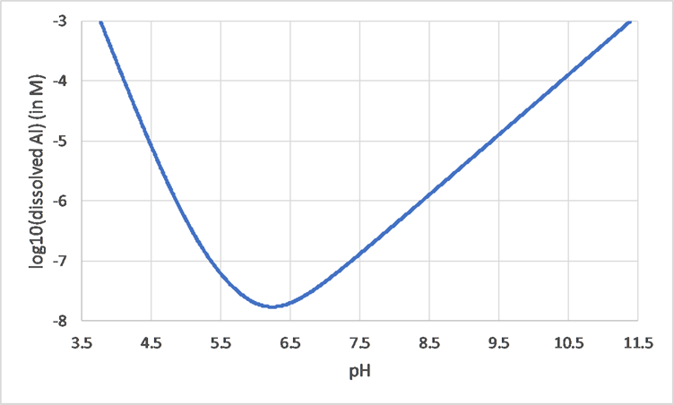
Many metals are amphoteric and have therefore a minimum solubility at a moderate pH, while dissolving more at both higher and lower pH-values. This can easily be seen in the case of Al: Figure 2 shows the concentration of dissolved Al as a function of pH (note log-scale for Y-axis). Around pH of 6.2, the solubility is at its minimum. At higher and lower pH-values, the solubility is (much) higher.

Figure 2. Soluble Al as function of pH. Data obtained using speciation program CHEAQS Next.

Speciation models can also help to understand differences in the growth of organisms or adverse effects on organisms, in different chemical solutions. For example, Figure 3 shows that changes in speciation of boron can be expected only between roughly pH 8 and 10.5, so when you observe a biological difference between pH 7 and 8, it is not likely that boron is the cause. Copper on the other hand (see Figure 4) does display differences in speciation between pH 7 and 8 so is a more likely cause of different biological behaviour.

Figure 3. Speciation of B as function of pH; concentration of boron was 1x10^-6 M. At higher concentrations, complexes with 2, 3, 4 or 5 B-ions can be formed at significant concentrations. Data obtained using speciation program CHEAQS Next.

Figure 4. Speciation of copper(II) as a function of pH; concentration of copper was 3x10^-8 M. At higher concentrations, complexes with 2 or 3 Cu(II)-ions can be formed at significant concentrations. Data obtained using speciation program CHEAQS Next.

Chemical behaviour: field situations

In field situations, the chemistry is usually much more complex than under laboratory conditions. Decomposition of organisms (including plants) results in a huge variety of organic compounds like fulvic acids, humic acids, proteins, amino acids, carbohydrates, etc. Many of these compounds interact strongly with cations, some also with anions or uncharged molecules. In addition, metals easily adsorb to clay and sand particles that are found everywhere in nature. To make it more complex, suspended matter can contain a high content of organic material which is also capable of binding cations.

For complexation by fulvic and humic acids, Tipping and co-workers have developed a unifying model (Tipping & Hurley, 1992; Tipping, 1994, 1998; Tipping, Lofts & Sonke, 2011). The most recent version, WHAM 7 (Tipping, Lofts & Sonke, 2011), is able to predict cation complexation by fulvic acids and humic acids over a wide range of chemical circumstances, despite the large difference in composition of these acids. This model is now incorporated in several speciation programs.

Suspended matter may be of organic or of inorganic character. Inorganic matter usually consists of (hydr)oxides of metals, such as Mn, Fe, Al, Si or Ti, and clay minerals. In practice, the (hydr)oxides and clays occur together, but the mutual proportions may differ dramatically depending on the source. Since the chemical properties of these metal (hydr)oxides clays are quite different, there is a huge variation in the chemical properties of inorganic suspended matter in different places and different times. As a consequence, modeling interactions between dissolved constituents and suspended inorganic matter is challenging. Only by measuring some properties of suspended inorganic matter, can modeling be applied successfully. For suspended organic matter, the variation in properties is also large and modelling is challenging.

Bioavailability

Speciation models are useful in understanding and assessing the bioavailability of metals and other elements in test media. Test media often contain substances like EDTA to keep metals in solution. EDTA-complexes in general are not bioavailable, so in addition to keeping metals in solution they also change their bioavailability. Models can calculate the speciation and help you to assess what is actually happening in a test medium. An often forgotten aspect is the influence of CO₂. CO₂ from the ambient atmosphere can enter a solution or carbonate in solution (if in excess over the equilibrium concentration) can escape to the atmosphere. The degree to which this exchange takes place, influences the pH of the solution as well as the amount of carbonate that stays in solution (carbonates are often poorly soluble).

Similarly, in field situations models can help to understand the bioavailability of elements. As stated above, the influence of DOC can nowadays be assessed properly in many situations, the influence of suspended matter remains more difficult to assess. Nevertheless models can deliver insights in seconds that otherwise can be obtained only with great difficulty.

Models

There are many speciation programs available and several of them are freely available. Usually they take a set of total concentrations as input, plus information about parameters such as pH, redox, concentration of organic carbon etc. Then the programs calculate the speciation and present them to the user. The equations cannot be solved analytically, so an iterative procedure is required. Although different numerical approaches are used, most programs construct a set of non-linear mass balance equations and solve them by simple or advanced mathematics. A complication in this procedure is that the equilibrium constants depend on the ionic strength of the solution, and that this ionic strength can only be calculated when the speciation is known. The same holds for the precipitation of solids. The procedure is shown in Figure 5.

Figure 5. Typical flow diagram of a speciation program.

Limitations

For modeling speciation, thermodynamic data is needed for all relevant equilibrium reactions. For many equilibria, this information is available, but not for all. This hampers the usefulness of speciation modeling. In addition, there can be large variations in the thermodynamic values found in the literature, resulting in uncertainty about the correct value. A factor of 10 between the highest and lowest values found is not an exception. This of course influences the reliability of speciation calculations. For many equilibria, the thermodynamic data is only available for the standard temperature of 25°C and no information is available to assess the data at other temperatures, although the effect of temperature can be quite strong. Also ionic strength has a high impact on equilibrium 'constants'; there are many methods available to correct for the effect of ionic strength, but most of them are at best semi-empirical. Simonin (2017) recently proposed a method with a solid theoretical basis; however, the data required for his method are available only for a few complexes so far.

More fundamentally, you should realize that speciation programs typically calculate the equilibrium situation, while some reactions are very slow and, more inportant, nature is in fact a very dynamic system and therefore never in equilibrium. If a system is close to equilibrium, speciation programs can often make a good assessment of the actual situation, but the more dynamic a system, the more care you should take in believing the programs' results. Nevertheless it is good to realise that a chemical system will always move towards the equilibrium situation, while organisms may move them away from equilibrium. Phototrophs are able to move a system away from its equilibrium situation whereas decomposers and heterotrophs generally help to move a system towards its equilibrium state.

References

Simonin , J.-P. (2017). Thermodynamic consistency in the modeling of speciation in self-complexing electrolytes. Ind. Eng. Chem. Res. 56, 9721-9733.

Tipping, E., Hurley, M.A. (1992). A unifying model of cation binding by humic substances. Geochimica et Cosmochimica Acta 56, 3627 - 3641.

Tipping, E. (1994). WHAM - A chemical equilibrium model and computer code for waters, sediments, and soils incorporating a discrete site/electrostatic model of ion-binding by humic substances. Computers & Geosciences 20, 973 - 1023.

Tipping, E. (1998). Humic Ion-Binding Model VI: An Improved Description of the Interactions of Protons and Metal Ions with Humic Substances. Aquatic Geochemistry 4, 3 - 48.

Tipping, E., Lofts, S., Sonke, J.E. (2011). Humic Ion-Binding Model VII: a revised parameterisation of cation-binding by humic substances. Environmental Chemistry 8, 228 - 235.

Further reading

Stumm, W., Morgan, J.J. (1981). Aquatic chemistry. John Wiley & Sons, New York.

More, F.M.M., Hering, J.G. (1993). Principles and Applications of Aquatic Chemistry. John Wiley & Sons, New York.

3.8.3. Question 1

Briefly describe what speciation models are.

---

3.8.3. Question 2

What are the factors determining speciation and how can these be accounted for?

---

3.8.3. Question 3

Give two examples of situations where speciation modeling can be useful.

---

3.8.4. Modeling exposure at ecological scales

In preparation