4.5: Availability and bioavailability

3.6. Availability and bioavailability

3.6.1. Definitions

Authors: Martina Vijver

Reviewer: Kees van Gestel, Ravi Naidu

Leaning objectives:

You should be able to:

• understand that bioavailability consists of three principle processes.
• understand that bioavailability is a dynamic concept.
• understand why bioavailability is important to explain uptake and effects, essential for a proper risk assessment of chemicals.

Keywords: Chemical availability, actual and potential uptake, toxico-kinetics, toxico-dynamics.

Introduction:

Although many environmental chemists, toxicologists, and engineers claim to know what bioavailability means, the term eludes a consensus definition. Bioavailability may be defined as that fraction of chemical present in the environment that is or may become available for biological uptake by passage across cell membranes.

Figure 1. Bioavailability relates to a series of processes, ranging from processes external of organisms, towards internal tissues, and fully internal to the biological response site. Redrawn from Ortega-Calvo et al. (2015) by Wilma IJzerman.

Bioavailability generally is approached from a process-oriented point of view within a toxicological framework, which is applicable to all types of chemicals (Figure 1).

The first process is chemical availability which can be defined as the fraction of the total concentration of chemicals present in an environmental compartment that contributes to the exposure of an organism. The total concentration in an environmental compartment is not necessarily involved in the exposure, as a smaller or larger fraction of the chemical may be bound to organic or inorganic components of the environment. Organic matter and clay particles, for instance, are important in binding chemicals (see section on Soil), while also the presence of cations and pH are important factors modifying the partitioning of chemicals between different environmental phases (see section on Metal speciation).

The second process is the actual or potential uptake, described as the toxicokinetics of a substance which reflects the development with time of its concentration on, and in, the organism (see section on Bioconcentration and kinetics modelling).

The third process describes the internal distribution of the substance leading to its interaction(s) at the cellular site of toxicity activation. This is sometimes referred to as toxico-availability and also includes the biochemical and physiological processes resulting from the effects of the chemical at the site of action.

Details on the bioavailability concept described above as well as how the physico-chemical interactions influencing each process are described in the sections on Metal speciation and Bioconcentration and kinetics modelling.

Figure 2. Bioavailability relates to a series of time frames, particularly in external processes (according to Ortega-Calvo et al. 2015).

Kinetics are involved in all three basic processes. The timeframe can vary from very brief (less than seconds) to very long in the order of hundreds of years. Figure 2 shows that some fractions of pollutants are present in soil or sediment, but may never contribute to the transport of chemicals that could reach the internal site during an organism's lifespan. The fractions with different desorption kinetics may relate to different experimental techniques to determine the relevant bioavailability metric.

Box 1: Illustration of how bioavailability influences our human fitness Iron deficiency occurs when a body has not enough iron to supply its needs. Iron is present in all cells of the human body and has several vital functions. It is a key component of the hemoglobin protein, carrying oxygen to the tissues from the lungs. Iron also plays an important role in oxidation/reduction reactions, which are crucial for the functioning of the cytochrome P450 enzymes that are responsible for the biotransformation of endogenic as well as xenobiotic chemicals. Iron deficiency therefore can interfere with these vital functions, leading to a lack of energy (feeling tired) and eventually to malfunctioning of muscles and the brain. In case of iron deficiency, the medical doctor will prescribe Fe-supplements and iron-rich food such as red meat and green leafy vegetables like spinach. Although this will lead to a higher intake of iron (after all exposure is higher), it does not necessarily lead to a higher uptake as here bioavailability becomes important. It is advised to avoid drinking milk or caffeinated drinks together with eating iron-rich products or supplements because both drinks will prevent the absorption of iron in the intestinal tract. Calcium ions abundant in milk will compete with iron ions for the same uptake sites, so excess calcium will reduce iron uptake. Carbonates and caffeine molecules, but also phytate (inositol polyphosphate) present in vegetables, will strongly bind the iron, also reducing its availability for uptake.

Figure 3. Bioavailability correction to estimate the HC5 copper concentration in relation to properties like dissolved organic carbon content and pH (Table 1) in order to estimate its risk in different water types (according to Vijver et al. 2008), in comparison to the 1.5 µg/L total dissolved Cu in surface waters as the current generic Dutch standard (horizontal line). Redrawn from Vijver et al. (2008) by Wilma Ijzerman

Bioavailability used in Risk Assessment

For regulatory purposes, it is necessary to use a straightforward approach to assess and prioritize contaminated sites based on their risk to human and environmental health. The bioavailability concept offers a scientific underpinned concept to be used in risk assessment. Examples for inorganic contaminants are the derived 2^nd tier models such as the Biotic Ligand Models, while for organic chemicals the Equilibrium Partitioning (E_qP) concept (see Box 2 in the section on Sorption) is applied.

A quantitative example is given for copper in different water types in Figure 3 and Table 1, in which water chemistry is explicitly accounted for to enable estimating the available copper concentration. The current Dutch generic quality target for surface waters is 1.5 µg/L total dissolved copper. The bioavailability-corrected risk limits (HC5) for different water types, in most cases, exceeded this generic quality target.

Table 1. Bioavailability adjusted Copper 5% Hazardous Concentration (HC5, potentially affecting <5% of relevant species) for different water types.

Water type description	no.	DOC (mg/L)	pH	Average HC5 (µg/L)
Large rivers	1	3.1 ± 0.9	7.7 ± 0.2	9.6 ± 2.9
Canals, lakes	2	8.4 ± 4.4	8.1 ± 0.4	35.0 ± 17.9
Streams, brooks	3	18.2 ± 4.3	7.4 ± 0.1	73.6 ± 18.9
Ditches	4	27.5 ± 12.2	6.9 ± 0.8	64.1 ± 34.5
Sandy springs	5	2.2 ± 1.0	6.7 ± 0.1	7.2 ± 3.1

When the calculated HC5 value is lower, this means that the bioavailability of copper is higher and hence at the same total copper concentration in water the risk is higher. The bioavailability-corrected HC5s for Cu differ significantly among water types. The lowest HC5 values were found for sandy springs (water type V) and large rivers (water type I), which appear to be sensitive water bodies. These differences can be explained from partitioning processes (chemical availability) and competition processes (the toxicokinetics step) on which the BLMs are based. Streams and brooks (water type III) have rather high total copper concentrations without any adverse effects, which can be attributed to the protective effect of relatively high dissolved organic carbon (DOC) concentrations and the neutral to basic pH causing a high binding of Cu to the DOC.

For risk managers, this water type specific risk approach can help to identify the priority in cleanup activities among sites having elevated copper concentrations. It remains possible that, for extreme environmental situations (e.g., extreme droughts and low water discharges or extreme rain fall and high runoff), combinations of the water chemistry parameters may result in calculated HC5 values that are even lower than the calculated average values. For the latter (important) reason, the generic quality target is more strict.

References

Hamelink, J., Landrum, P.F., Bergman, H., Benson, W.H. (1994) Bioavailability: physical, chemical, and biological interactions, CRC Press.

Ortega-Calvo, J.J., Harmsen, J., Parsons, J.R., Semple, K.T., Aitken, M.D., Ajao, C., Eadsforth, C., Galay-Burgos, M., Naidu, R., Oliver, R., Peijnenburg, W.J.G.M., Römbke, J., Streck, G., Versonnen, B. (2015) From bioavailability science to regulation of organic chemicals. Environmental Science and Technology 49, 10255−10264.

Vijver, M.G., de Koning, A., Peijnenburg, W.J.G.M. (2008) Uncertainty of water type-specific hazardous copper concentrations derived with biotic ligand models. Environmental Toxicology and Chemistry 27, 2311-2319.

3.6.1. Question 1

What are the three processes that define bioavailability?

---

3.6.1. Question 2

Explain how metal uptake changes when high concentrations of dissolved organic matter are in the exposure medium.

---

3.6.1. Question 3

Explain why bioavailability is a dynamic concept.

---

3.6.2. Assessing available concentrations of organic chemicals

Author: Jose Julio Ortega-Calvo

Reviewers: John Parsons, Gerard Cornelissen

Learning objectives:

You should be able to:

• define the concept of freely dissolved concentrations and fast-desorbing fractions of organic chemicals in soil and sediment, as indicators of their bioavailability
• understand how to determine bioavailable concentrations with the use of passive sampling
• understand how to determine fast-desorbing fractions with desorption extraction methods.

Keywords: Bioavailability, Freely-dissolved concentration, Desorption, Passive sampling, Infinite sink

Introduction: Bioavailability through the water phase

In many exposure scenarios involving organic chemicals, ranging from a bacterial cell to a fish, or from a sediment bed to a soil profile, the organisms experience the pollution through the water phase. Even when this is not the case, for example when uptake is from sediment consumed as food, the aqueous concentration may be a good indicator of the bioavailable concentration, since ultimately a chemical equilibrium will be established between the solid phase, the aqueous phase (possibly in the intestine), and the organism. Thus, taking an aqueous sample from a given environment, and determining the concentration of a certain chemical with the appropriate analytical equipment seems a straightforward approach to assess bioavailability. However, especially for hydrophobic chemicals, which tend to remain sorbed to solid surfaces (see sections on Relevant chemical properties and Sorption of organic chemicals), the determination of the chemicals present in the aqueous phase, as a way to assess bioavailability, has represented a significant challenge to environmental organic chemistry. The phase exchange among different compartments often leads to equilibrium aqueous concentrations that are very low, because most of the chemicals remain associated to the solids, and after sustained exposure, to the biota. These freely dissolved concentrations (C_free) are very useful to determine bioavailability, as they represent the "tip of the iceberg" under equilibrium exposure, and are what organisms "see" (Figure 1, left). Similarly to the balance between gravity and buoyancy forces leading to iceberg flotation up to a certain level, C_free is determined by the equilibrium between sorption and desorption, and connected to the concentration of the sorbed chemical (C_sorbed) through a partitioning coefficient.

Biological uptake may also result in the fast removal of the chemical from the aqueous phase, and thus in further desorption from the solids, so equilibrium is never achieved, and actual aqueous concentrations are much lower than the equilibrium C_free (or even close to zero). In these situations, bioavailability is driven by the desorption kinetics of the chemical. Usually, desorption occurs as a biphasic process, where a fast desorption phase, occurring during a few hours or days, is followed by a much slower phase, taking months or even years. Therefore, for scenarios involving rapid exposures, or for studies on coupled desorption/biodegradation, the fast-desorbing fraction of the chemicals (F_fast) can be used to determine bioavailability. This fraction is often referred to as the bioaccessible fraction. Following the iceberg analogy (Figure 1, right), F_fast would constitute the upper iceberg fraction rapidly melting by sun irradiation, with a very minimal "visible" surface (representing the desorbed chemical in the aqueous solution, which is quickly removed by biological uptake). The slowly desorbing -or melting- fraction, F_slow, would remain in the sorbed state, within a given time span, having little interactions with the biota.

Figure 1. The magnitude of C_free, determined by the sorption/desorption equilibrium (similarly to a floating iceberg, left), can correspond to a minimal fraction of the total pollutant mass, but may constitute the main driver for bioavailability (and risk) in equilibrium exposure scenarios. In non-equilibrium conditions (right, in analogy, a melting iceberg exposed to irradiation to sun), the fraction of sorbed chemical that can be rapidly mobilized, F_fast, can be taken as an estimate of bioavailability.

Determining bioavailability with passive sampling methods

C_free can be determined with a passive sampler, in the form of polymer-coated fibers or sheets (membranes) made of a variety of polymers, which establish an additional sorption equilibrium with the aqueous phase in contact with the soil or sediment (Jonker et al., 2018). Depending on the analytes of interest, different polymers, such as polydimethylsiloxane (PDMS) or polyethylene (PE), are used in passive samplers. The passive sampler, enriched in the analyte (similarly to the floating iceberg in Figure 1, left, where C_sorbed in this case is the concentration in the passive sampler), can be used in this way to determine indirectly the pollutant concentration present in the aqueous phase, even at very low concentrations, though the appropriate distribution ratio between sampler and water. In bioavailability estimations, passive sampling is designed for equilibrium and non-depletive conditions. This means that the amount of chemical sampled does not alter the solid-water equilibrium, i.e., it is essential that C_free is not affected significantly by the sampler. Equilibrium achievement is critical, and it may take days or weeks.

C_free can be calculated from the concentration of the pollutant in the passive sample polymer at equilibrium (C_p), and the polymer-to-water partitioning coefficient (K_pw):

C_free values can be the basis of predictions for bioaccumulation that use the equilibrium partitioning approach, either directly or through a bioconcentration factor, and for sediment toxicity in conjunction with actual toxicity tests. Passive sampling methods are well suited for contaminated sediments, and they have already been implemented in regulatory environmental assessments based on bioavailability (Burkhard et al., 2017).

Determining bioavailability with desorption extraction methods

The determination of F_fast can be achieved with the use of methods that trap the desorbed chemical once it appears in the aqueous phase. Far from equilibrium conditions, desorption is driven to its maximum rate by placing a material in the aqueous phase that acts as an infinite sink (comparable to the sun irradiation of a melting iceberg in Figure 1, right). The most accepted materials for these desorption extraction methods are Tenax, a sorptive resin, and cyclodextrin, a solubilizing agent (ISO, 2018). These methods allow a permanent aqueous chemical concentration of almost zero, and therefore, sorption of the chemical back to the soil or sediment can be neglected. Several extraction steps can be used, covering a variable time span, which depends on the environmental sample.

The following first-order, two-compartment kinetic model can be used to analyze desorption extraction data:

In this equation, S_t and S_o (mg) are the soil-sorbed amounts of the chemical at time t (h) and at the start of the experiment, respectively. F_fast and F_slow are the fast- and slow-desorbing fractions, and k_fastand k_slow(h^-1) are the rate constants of fast and slow desorption, respectively. To calculate the values of the different constants and fractions (F_fast, F_slow, k_fast, and k_slow) exponential curve fitting can be used. The ln form of the equation can be used to simplify curve fitting.

Once the desorption kinetics are known, the method can be simplified for a series of samples, by using single time point-extractions. A time period of 20 h has been suggested as a sufficient time period to approximate F_fast. It is highly convenient for operational reasons (ISO, 2018), but indicative at best, since the time needed to extract Ffast tends to vary between chemicals and soils/sediments.

References

Burkhard, L.P., Mount, D.,R., Burgess, R.,M. (2017). Developing Sediment Remediation Goals at Superfund Sites Based on Pore Water for the Protection of Benthic Organisms from Direct Toxicity to Nonionic Organic Contaminants EPA/600/R 15/289; U.S. Environmental Protection Agency Office of Research and Development: Washington, DC.

ISO (2018). Technical Committee ISO/TC 190 Soil quality - Environmental availability of non-polar organic compounds - Determination of the potentially bioavailable fraction and the non-bioavailable fraction using a strong adsorbent or complexing agent; International Organization for Standardization: Geneva, Switzerland.

Jonker, M.T.O., van der Heijden, S.A., Adelman, D., Apell, J.N., Burgess, R.M., Choi, Y., Fernandez, L.A., Flavetta, G.M., Ghosh, U., Gschwend, P.M., Hale, S.E., Jalalizadeh, M., Khairy, M., Lampi, M.A., Lao, W., Lohmann, R., Lydy, M.J., Maruya, K.A., Nutile, S.,A., Oen, A.M.P., Rakowska, M.I., Reible, D., Rusina, T.P., Smedes, F., Wu, Y. (2018) Advancing the use of passive sampling in risk assessment and management of sediments contaminated with hydrophobic organic chemicals: results of an international ex situ passive sampling interlaboratory comparison. Environmental Science & Technology 52 (6), 3574-3582.

3.6.2. Question 1

Describe why the freely dissolved concentration is often used as an indicator of the bioavailability of organic chemicals in soil and sediment.

---

3.6.2. Question 2

What is passive sampling and how can this be used to determine the bioavailable concentrations of chemicals in soil or sediment?

---

3.6.2. Question 3

What is the meant by fast-desorbing fraction of a chemical in soil or sediment and how can this be determined with desorption extraction methods?

---

3.6.3. Assessing available metal concentrations

Authors: Kees van Gestel

Reviewer: Martina Vijver, Steve Lofts

Leaning objectives:

You should be able to:

• mention different methods for assessing chemically available metal fractions in soils and sediments.
• indicate the relative binding strengths of metals extracted with the different methods or in different steps of a sequential extraction procedure.
• explain the pros and cons of chemical extraction methods for assessing metal (bio)availability in soils and sediments.

Keywords: Chemical availability, actual and potential uptake, toxicokinetics, toxicodynamics.

Introduction:

Total concentrations are not very informative about the availability of metals in soils or sediments. Fate and behavior of metals - in general terms mobility - as well as biological uptake and toxicity is highly determined by their speciation. Speciation describes the partitioning of a metal among the various forms in which it may exist (see section on Metal speciation). For assessing the risk of metals to man and the environment, speciation therefore is highly relevant as it may determine their availability for uptake and effects in organisms. Several tools have been developed to determine available metal concentrations or their speciation in soils and sediments. As indicated in the section on Availability and bioavailability, such chemical methods are just indicative, and to a large extent ignore dynamics of availability. Moreover, availability is also influenced by biological processes, with abiotic-biotic interactions influencing the bioavailability process being species- and often even life-stage specific. Nevertheless, chemical extractions may provide useful information to predict or estimate the potential risks of metals and therefore are preferred over the determination of total metal concentrations.

The available methods include:

1. Porewater extraction
2. Extractions with water
3. Extractions with diluted salts
4. Extractions with chelating agents
5. Extractions with diluted acids
6. Sequential extractions using a series of different extraction solutions
7. Passive sampling methods

Porewater extraction probably best approaches the readily available fraction of metals in soil, which drives mobility and is the fraction of metals experienced directly by many organisms exposed. In general, pore water is extracted from soil or sediment by centrifugation, and filtration over a 0.45 µm (or 0.22 µm) filter to remove larger particles and perhaps some of the dissolved organic matter. Filtration, however, will not remove all complexes, making it impossible to determine solely the dissolved metal fraction in the pore water. Nevertheless, porewater metal concentrations have been shown to have significant correlations with metal uptake (e.g. for copper uptake by barley and tomato by Zhao et al., 2006) and to be useful for predicting toxic threshold concentrations of metals, with correction for pH (e.g. for nickel toxicity to tomato and barley by Rooney et al., 2007).

Extraction with water simulates the immediately available fraction, so the fraction present in the soil solution or pore water. By extracting soil with water, the pore water however, is diluted, which on one hand may facilitate metal analysis by creating larger volumes of solution, but on the other hand may lead to differences between measured and actual metal concentrations in the pore water as it may impact chemical equilibria.

Extraction with diluted salts aims to determine the fraction of metal that is easily available or may become available as it is in the exchangeable form. This refers to cationic metals that may be bound to the negatively charged soil particles (see section on Soil). Buffered salt solutions, for instance 1 M NH₄-acetate at pH 4.8 (with acetic acid) or at pH 7, may under- or overestimate available metal concentrations because of their interference with soil pH. Unbuffered salt solutions therefore are more widely used and may for instance include 0.001 or 0.01 M CaCl₂, 0.1 M NaNO₃ or 1 M NH₄NO₃ (Gupta and Aten, 1993; Novozamsky et al., 1993). Gupta and Aten (1993) showed good correlations between the uptake of some metals in plants and 0.1 M NaNO₃ extractable concentrations in soil, while Novozamsky et al. (1993) found similar well-fitting correlations using 0.01 M CaCl₂. The latter method also seemed well capable of predicting metal uptake in soil invertebrates, and therefore has been more widely accepted for predicting metal availability in soil ecotoxicology. Figure 1 (Zhang et al., 2019) provides an example with the correlation between Pb toxicity to enchytraeid worms in different soils and 0.01 M CaCl₂ extractable concentrations.

Extractions with water (including porewater) and dilute salts are most accurately described as measures of the chemical solubility of the metal in the soil. The values obtained can be useful indicators of the relative metal reactivity across soils, but tend to be less useful for bioavailability assessment, unless the soils under consideration have a narrow range of soil properties. This is because the solutions obtained from such soils themselves have varying chemical properties (e.g. pH, DOC concentration) which are likely to affect the availability of the measured metal to organisms.

Figure 1. Effects of Pb(NO₃)₂ on the reproduction of Enchytraeus crypticus after three weeks exposure in six natural soils. Pb concentrations are expressed as total (A) and 0.01 M CaCl₂ extractable concentrations in soil (B). Lines show the fit of a logistic dose-response curve. When expressed on the basis of 0.01 M CaCl₂ extrable concentrations, dose-response curves did not significantly differ and a single curve is shown. Data taken from Zhang et al. (2019).

Extraction with chelating agents, such as EDTA (0.01-0.05 M) or DTPA (0.005 M) (as their sodium or ammonium salts), aims at assessing the availability of metals for plants. Many plants have the ability to actively affect metal speciation in the soil by producing root exudates. These extractants may form very stable water-soluble complexes with many different polyvalent cationic metals. It should be noted that the large variation in plant species and corresponding physiologies as well as their interactions with symbiotic microorganisms (e.g. mycorrhizal fungi) make that there is no single extraction method is capable of properly predicting metal availability to all plant species.

Extraction with diluted acids has been advocated for predicting the potentially available fraction of metals in soils, so the fraction that may become available in the long run. It is a quite rigorous extraction method that can be executed in a robust way. Metal concentrations determined by extracting soils with 0.43 M HNO₃ showed very good correlation with oral bioaccessible concentrations (Rodrigues et al., 2013), probably because it to some degree simulates metal release under acidic stomach conditions.

Both extraction methods with chelating agents and diluted acid may also dissolve solids, such as carbonates and Fe- and Al-oxides. This raises concerns as to the interpretation of results of these extraction systems, and especially to their generalization to different soil-plant systems (Novozamsky et al., 1993). The extractions with chelating agents and dilute acids are considered methods to estimate the 'geochemically active' metal in soil - the pool of adsorbed metal that can participate in solid-solution adsorption/desorption and exchange equilibria on timescales of hours to days. This pool, along with the basic soil properties such as pH etc., also controls the readily available concentrations obtained with water/weak salt/porewater extraction. From the bioavailability point of view, these extractions tend to be most useful as inputs to bioavailability/toxicity models such as that of Lofts et al. (2014), which take further account of the effects of metal speciation and soil chemistry on metal bioavailability to environmental organisms.

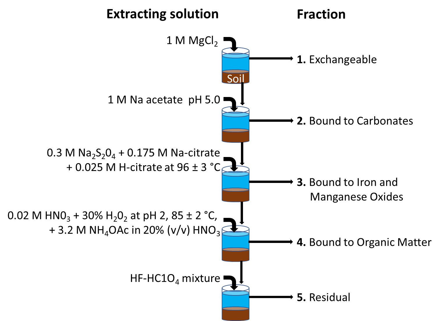
Sequential extraction brings together different extraction methods, and aims to determining either how strongly metals are retained or to which components of the solid phase they are bound in soils or sediments. This allows to determine how metals are bound to different fractions within the same soil or sediment, and allows interpretation to the bioavailability dynamics. By far the most widely used method of sequential extraction is the one proposed by Tessier et al. (1979). Five fractions are distinguished, indicating how metals are interacting with soil or sediment components: see Figure 2.

Where the Tessier method aims at assessing the environmental availability of metals in soils and sediments, similar sequential extraction methods have also been developed for assessing the potential availability of metals for humans (bioaccessibility) following gut passage of soil particles (see e.g. Basta and Gradwohl, 2000).

Figure 2. Schematic presentation of the sequential extraction of soil or sediment samples following the method of Tessier et al. (1979). The fractions obtained give an indication of the sites where metals are bound in the soil or sediment, and represent also an increasing binding strength, going from exchangeable to residual. Source: Kees van Gestel.

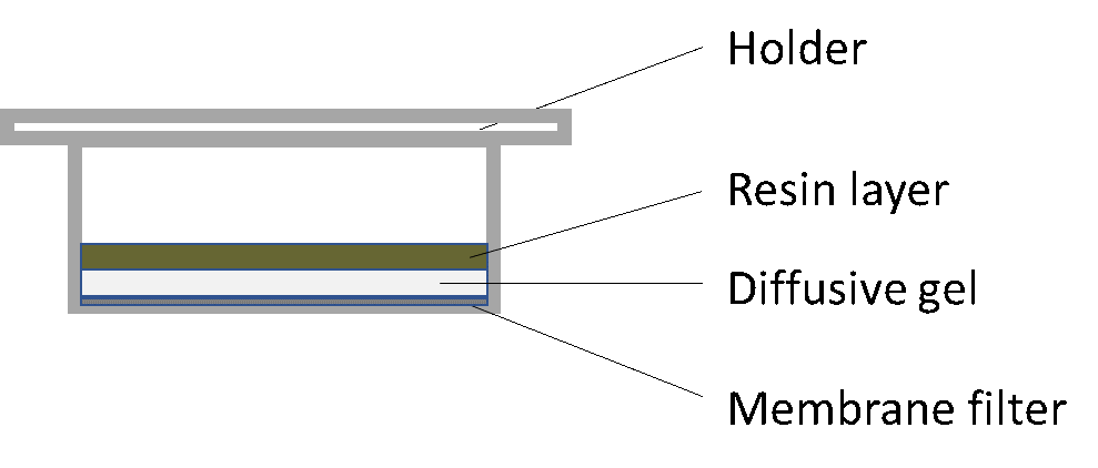
Passive sampling may also be applied to assess available metal concentrations. The best known method is that of Diffusive Gradients in Thin films (DGT), developed by Zhang et al. (1998). In this method, a resin (Chelex) with high affinity for metals is placed in a device and covered with a diffusive gel and a 0.45 µm cellulose nitrate membrane (Figure 3). The membrane is brought into contact with the soil. Metals dissolved in the soil solution will diffuse through a membrane and diffusive gel and bind to the resin. Based on the thickness of the membrane and gel and the contact time with the soil, the metal concentration in the pore water can be calculated from the amount of metal accumulated in the resin. The method may be indicative of available metal concentrations in soils and sediments, but can only work effectively when soil is sufficiently moist to guarantee optimal diffusion of metals to the resin. For the same reasons, the method probably is better suited for assessing the availability of metals to plants than to invertebrates, especially for animals that are not in continuous contact with the soil solution.

Figure 3. Device used in the Diffusive Gradients in Thin film (DGT) method for determining available metal concentrations in soil and sediment (adapted from Zhang et al., 1998). The device is placed on the soil or sediment in such a way that the membrane filter makes contact with the porewater. Metals may diffuse from the porewater to the resin layer. See text for further explanation.

Several of the above described methods have been adopted by the International Standardization Organization (ISO) in (draft) standardized test guidelines for assessing available metal fractions in soils, sediments and waste materials, e.g. to assess the potential for leaching to groundwater or their potential bioaccessibility. This includes e.g. ISO/TS 21268-1 (2007) "Soil quality - Leaching procedures for subsequent chemical and ecotoxicological testing of soil and soil materials - Part 1: Batch test using a liquid to solid ratio of 2 l/kg dry matter", ISO 19730 (2008) "Soil quality -Extraction of trace elements from soil using ammonium nitrate solution" and ISO 17586 (2016) "Soil quality -- Extraction of trace elements using dilute nitric acid".

References:

Basta, N., Gradwohl, R. (2000). Estimation of Cd, Pb, and Zn bioavailability in smelter-contaminated soils by a sequential extraction procedure. Journal of Soil Contamination 9, 149-164.

Gupta, S.K., Aten, C. (1993). Comparison and evaluation of extraction media and their suitability in a simple model to predict the biological relevance of heavy metal concentrations in contaminated soils. International Journal of Environmental Analytical Chemistry 51, 25-46.

Lofts, S., Spurgeon, D.J., Svendsen, C., Tipping, E. (2004). Deriving soil critical limits for Cu, Zn, Cd, and Pb: A method based on free ion concentrations. Environmental Science and Technology 38, 3623-3631.

Novozamsky, I., Lexmond, Th.M., Houba, V.J.G. (1993). A single extraction procedure of soil for evaluation of uptake of some heavy metals by plants. International Journal of Environmental Analytical Chemistry 51, 47-58.

Rodrigues, S.M., Cruz, N., Coelho, C., Henriques, B., Carvalho, L., Duarte, A.C., Pereira, E., Römkens, P.F. (2013). Risk assessment for Cd, Cu, Pb and Zn in urban soils: chemical availability as the central concept. Environmental Pollution 183, 234-242.

Rooney, C.P., Zhao, F.-J., McGrath, S.P. (2007). Phytotoxicity of nickel in a range of European soils: Influence of soil properties, Ni solubility and speciation. Environmental Pollution 145, 596-605.

Tessier, A., Campbell, P.G.C., Bisson, M. (1979). Sequential extraction procedure for the speciation of particulate trace metals. Analytical Chemistry 51, 844-851.

Zhang, H., Davison, W., Knight, B., McGrath, S. (1998). In situ measurements of solution concentrations and fluxes of trace metals in soils using DGT. Environmental Science and Technology 32, 704-710.

Zhang, L., Verweij, R.A., Van Gestel, C.A.M. (2019). Effect of soil properties on Pb bioavailability and toxicity to the soil invertebrate Enchytraeus crypticus. Chemosphere 217, 9-17.

Zhao, F.J., Rooney, C.P., Zhang, H., McGrath, S.P. (2006). Comparison of soil solution speciation and diffusive gradients in thin-films measurement as an indicator of copper bioavailability to plants. Environmental Toxicology and Chemistry 25, 733-742.

3.6.3. Question 1

Which metal fractions are extracted with the Tessier method, and what does that say about metal availability?

---

3.6.3. Question 2

Why is porewater extraction to be preferred above water extraction?

---

3.6.3. Question 3

What is the principle of the DGT passive sampling method, and why does it not work for fairly dry soils?

---

3.6.3. Question 4

Which method may give the best estimate of potentially available metals for oral uptake by mammals?

---

3.6.3. Question 5

What are the pros and cons of chemical extraction methods for assessing the availability of metals in soils or sediments

---