4.3: Toxicity Testing

4.3. Toxicity testing

Author: Kees van Gestel

Reviewer: Michiel Kraak

Learning objectives:

You should be able to

• Mention the two general types of endpoints in toxicity tests
• Mention the main groups of test organisms used in environmental toxicology
• Mention different criteria determining the validity of toxicity tests
• Explain why toxicity testing may need a negative and a positive control

Keywords: single-species toxicity tests, test species selection, concentration-response relationships, endpoints, bioaccumulation testing, epidemiology, standardization, quality control, transcriptomics, metabolomics,

Introduction

Laboratory toxicity tests may provide insight into the potential of chemicals to bioaccumulate in organisms and into their hazard, the latter usually being expressed as toxicity values derived from concentration-response relationships. Section 4.3.1 on Bioaccumulation testing describes how to perform tests to assess the bioaccumulation potential of chemicals in aquatic and terrestrial organisms, and under static and dynamic exposure conditions. Basic to toxicity testing is the establishment of a concentration-response relationship, which relates the endpoint measured in the test organisms to exposure concentrations. Section 4.3.2 on Concentration-response relationships elaborates on the calculation of the relevant toxicity parameters like the median lethal concentration (LC₅₀) and the medium effective concentration (EC₅₀) from such toxicity tests. It also discusses the pros and cons of different methods for analyzing data from toxicity tests.

Several issues have to be addressed when designing toxicity tests that should enable assessing the environmental or human health hazard of chemicals. This concerns among others the selection of test organisms (see section 4.3.4 on the Selection of test organisms for ecotoxicity testing), exposure media, test conditions, test duration and endpoints, but also requires clear criteria for checking the quality of toxicity tests performed (see below). Different whole organism endpoints that are commonly used in standard toxicity tests, like survival, growth, reproduction or avoidance behavior, are discussed in section 4.3.3 on Endpoints. The sections 4.3.4 to 4.3.7 are focusing on the selection and performance of tests with organisms representative of aquatic and terrestrial ecosystems. This includes microorganisms (section 4.3.6), plants (section 4.3.5), invertebrates (section 4.3.4) and vertebrate test organisms (e.g. fish: section 4.3.4 on ecotoxicity tests, and birds: section 4.3.7). Testing of vertebrates, including fish (section 4.3.4) and birds (section 4.3.7), is subject to strict regulations, aimed at reducing the use of test animals. Data on the potential hazard of chemicals to human health therefore preferably have to be obtained in other ways, like by using in vitro test methods (section 4.3.8), by using data from post-registration monitoring of exposed humans (section 4.3.9 on Human toxicity testing), or from epidemiological analysis on exposed humans (section 4.3.10).

Inclusion of novel endpoints in toxicity testing

Traditionally, toxicity tests focus on whole organism endpoints, with survival, growth and reproduction being the most measured parameters (section 4.3.3). In case of vertebrate toxicity testing, also other endpoints may be used addressing effects at the level of organs or tissues (section 4.3.9 on human toxicity testing). Behavioural (e.g. avoidance behavior) and biochemical endpoints, like enzyme activity, are also regularly included in toxicity testing with vertebrates and invertebrates (sections 4.3.3, 4.3.4, 4.3.7, 4.3.9).

With the rise of molecular biology, novel techniques have become available that may provide additional information on the effects of chemicals. Molecular tools may, for instance, be applied in molecular epidemiology (section 4.3.11) to find causal relationships between health effects and the exposure to chemicals. Toxicity testing may also use gene expression responses (transcriptomics; section 4.3.12) or changes in metabolism (metabolomics; section 4.3.13) in relation to chemical exposures to help unraveling the mechanism(s) of action of chemicals. A major challenge still is to explain whole organism effects from such molecular responses.

Standardization of tests

The standardization of tests is organized by international bodies like the Organization for Economic Co-operation and Development (OECD), the International Standardization Organization (ISO), and ASTM International (formerly known as the American Society for Testing and Materials). Standardization aims at reducing variation in test outcomes by carefully describing the methods for culturing and handling the test organisms, the procedures for performing the test, the properties and composition of test media, the exposure conditions and the analysis of the data. Standardized test guidelines are usually based on extensive testing of a method by different laboratories in a so-called round-robin test.

Regulatory bodies generally require that toxicity tests supporting the registration of new chemicals are performed according to internationally standardized test guidelines. In Europe, for instance, all toxicity tests submitted within the framework of REACH have to be performed according to the OECD guidelines for the testing of chemicals (see section on Regulation of chemicals).

Quality control of toxicity tests

Since toxicity tests are performed with living organisms, this inevitably leads to (biological) variation in outcomes. Coping with this variation requires the use of sufficient replication, careful test designs and good choice of endpoints (section 4.3.3) to enable proper estimates of relevant toxicity data.

In order to control the quality of the outcome of toxicity tests, several criteria have been developed, which mainly apply to the performance of the test organisms in the non-exposed controls. These criteria may e.g. require a minimum % survival of control organisms, a minimum growth rate or number of offspring being produced by the controls and limited variation (e.g. <30%) of the replicate control growth or reproduction data (sections 4.3.4, 4.3.5, 4.3.6, 4.3.7). When tests do not meet these criteria, the outcome is prone to doubts, as for instance a poor control survival will make it hard to draw sound conclusions on the effect of the test chemical on this endpoint. As a consequence, tests that do not meet these validity criteria may not be accepted by other scientists and by regulatory authorities.

In case the test chemical is added to the test medium using a solvent, toxicity tests should also include a solvent control, in addition to a regular non-exposed control (see section 4.3.4 on the selection of test organisms for ecotoxicity testing). In case the response in the solvent control differs significantly from that in the negative control, the solvent control will be used as the control for analyzing the effects of the test chemical. The negative control will then only be used to check if the validity criteria have been met and to monitor the condition of the test organisms. In case the responses in the negative control and the solvent control do not differ significantly, both controls can be pooled for the data analysis.

Most test guidelines also require frequent testing of a positive control, a chemical with known toxicity, to check if the long-term culturing of the test organisms does not lead to changes in their sensitivity.

4.3. Question 1

What are the main endpoints in toxicity testing?

---

4.3. Question 2

Which are the main groups of organisms used in toxicity testing?

---

4.3. Question 3

Why is standardization of methods for toxicity testing required?

---

4.3. Question 4

Which elements are included in the quality control of toxicity tests?

---

4.3.1. Bioaccumulation testing

Author: Kees van Gestel

Reviewers: Joop Hermens, Michiel Kraak, Susana Loureiro

Learning objectives:

You should be able to

• describe methods for determining the bioaccumulation of chemicals in terrestrial and aquatic organisms
• describe a test design suitable for assessing the bioaccumulation kinetics of chemicals in organisms
• mention the pros and cons of static and dynamic bioaccumulation tests

Keywords: bioconcentration, bioaccumulation, uptake and elimination kinetics, test methods, soil, water

Bioaccumulation is defined as the uptake of chemicals in organisms from the environment. The degree of bioaccumulation is usually indicated by the bioconcentration factor (BCF) in case the exposure is via water, or the biota-to-soil/sediment accumulation factor (BSAF) for exposure in soil or sediment (see section on Bioaccumulation).

Because of the potential risk for food-chain transfer, experimental determination of the bioaccumulation potential of chemicals is usually required in case of a high lipophilicity (log K_ow > 3), unless the chemical has a very low persistency. For very persistent chemicals, experimental determination of bioaccumulation potential may already be triggered at log K_ow > 2. The experimental determination of BCF and BSAF values makes use of static or dynamic exposure systems.

In static tests, the medium is dosed once with the test chemical, and organisms are exposed for a certain period of time after which both the organisms and the test medium are analyzed for the test chemical. The BCF or BSAF are calculated from the measured concentrations. There are a few concerns with this way of bioaccumulation testing.

First, exposure concentrations may decrease during the test, e.g. due to (bio)degradation, volatilization, sorption to the walls of the test container, or uptake of the test compound by the test organisms. As a consequence, the concentration in the test medium measured at the start of the test may not be indicative of the actual exposure during the test. To take this into account, exposure concentrations can be measured at the start and the end of the test and also at some intermediate time points. Body concentrations in the test organisms may then be related to time-weighted-average (TWA) exposure concentrations. Alternatively, to overcome the problem of decreasing concentrations in aquatic test systems, continuous flow systems or passive dosing techniques can be applied. Such methods, however, are not applicable to soil or sediment tests, where repeated transfer of organisms to freshly spiked medium is the only way to guarantee more or less constant exposure concentrations in case of rapidly degrading compounds. To avoid that the uptake of the test chemical in test organisms leads to decreasing exposure concentrations, the amount of biomass per volume or mass of test medium should be sufficiently low.

Second, it is uncertain whether at the end of the exposure period steady state or equilibrium is reached. If this is not the case, the resulting BSAF or BCF values may underestimate the bioaccumulation potential of the chemical. To tackle this problem, a dynamic test may be run to assess the uptake and elimination rate constants to derive a BSAF or BCF values using uptake and elimination rate constants (see below).

Such uncertainties also apply to BCF and BSAF values obtained by analyzing organisms collected from the field and comparing body concentrations with exposure levels in the environment. Using data from field-exposed organisms on one hand have large uncertainty as it remains unclear whether equilibrium was reached, on the other hand they to do reflect exposure over time under fluctuating but realistic exposure conditions.

Dynamic tests, also indicated as uptake/elimination or toxicokinetic tests, may overcome some, but not all, of the disadvantages of static tests. In dynamic tests, organisms are exposed for a certain period of time in spiked medium to assess the uptake of the chemical, after which they are transferred to clean medium for determining the elimination of the chemical. During both the uptake and the elimination phase, at different points in time, organisms are sampled and analyzed for the test chemical. The medium is also sampled frequently to check for a possible decline of the exposure concentration during the uptake phase. Also in dynamic tests, keeping exposure concentrations constant as much as possible is a major challenge, requiring frequent renewal (see above).

Toxicokinetic tests should also include controls, consisting of test organisms incubated in the clean medium and transferred to clean medium at the same time the organisms from the treated medium are transferred. Such controls may help identifying possible irregularities in the test, such as poor health of the test organisms or unexpected (cross)contamination occurring during the test.

The concentrations of the chemical measured in the test organisms are plotted against the exposure time, and a first-order one-compartment model is fitted to the data to estimate the uptake and elimination rate constants. The (dynamic) BSAF or BCF value is then determined as the ratio of the uptake and elimination rate constants (see section on Bioconcentration and kinetic models).

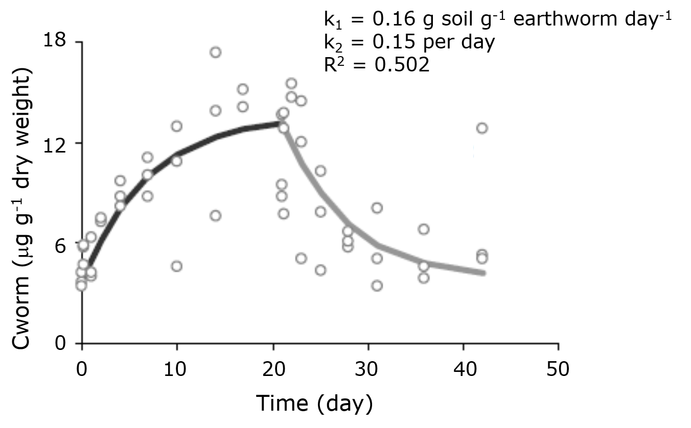
In a toxicokinetics test, usually replicate samples are taken at each point in time, both during the uptake and the elimination phase. The frequency of sampling may be higher at the beginning than at the end of both phases: a typical sampling scheme is shown in Figure 1. Since the analysis of toxicokinetics data using the one-compartment model is regression based, it is generally preferred to have more points in time rather than having many replicates per sampling time. From that perspective, often no more than 3-4 replicates are used per sampling time, and 5-6 sampling times for the uptake and elimination phases each.

Figure 1. Sampling scheme of a toxicokinetics test for assessing the uptake and elimination kinetics of chemicals in earthworms. During the 21-day uptake phase, the earthworms are individually exposed to a test chemical in soil, and at regular intervals three earthworms are sampled. After 21 days, the remaining earthworms are transferred to clean soil for the 21-day elimination period, in which again three replicate earthworms are sampled at regular points in time for measuring the body concentrations of the chemical. Also the soil is analyzed at different points in time (marked with X in the Medium row). Drawn by the author.

Preferably, replicates are independent, so destructively sampled at a specific sampling point. Especially in aquatic ecotoxicology, mass exposures are sometimes used, having all test organisms in one or few replicate test containers. In this case, at each sampling time some replicate organisms are taken from the test container(s), and at the end of the uptake phase all organisms are transferred to (a) container(s) with clean medium.

Figure 2 shows the result of a test on the uptake and elimination kinetics of molybdenum in the earthworm Eisenia andrei. From the ratio of the uptake rate constant (k₁) and elimination rate constant (k₂) a BSAF of approx. 1.0 could be calculated, suggesting a low bioaccumulation potential of Mo in earthworms in the soil tested.

Figure 2. Uptake and elimination kinetics of molybdenum in Eisenia andrei exposed in an artificial soil spiked with a nominal Mo concentration of 10 µg g^-1 dry soil. Dots represent measured internal Mo concentrations. Curves were estimated by a one-compartment model (see section on Bioconcentration and kinetic models). Parameters: k₁ = uptake rate constant [g_soil/g_worm/d], k₂ = elimination rate constant [d^-1]. Adapted from Diez-Ortiz et al. (2010).

Another way of assessing the bioaccumulation potential of chemicals in organisms includes the use of radiolabeled chemicals, which may facilitate easy detection of the test chemical. The use of radiolabeled chemicals may however, overestimate bioaccumulation potential when no distinction is made between the parent compound and potential metabolites. In case of metals, stable isotopes may also offer an opportunity to assess bioaccumulation potential. Such an approach was also applied to distinguish the role of dissolved (ionic) Zn in the bioaccumulation of Zn in earthworms from ZnO nanoparticles. Earthworms were exposed to soils spiked with mixtures of ⁶⁴ZnCl₂ and ⁶⁸ZnO nanoparticles. The results showed that dissolution of the nanoparticles was fast and that the earthworms mainly accumulated Zn present in ionic form in the soil solution (Laycock et al., 2017).

Standard test guidelines for assessing the bioaccumulation (kinetics) of chemicals have been published by the Organization for Economic Cooperation and Development (OECD) for sediment-dwelling oligochaetes (OECD, 2008), for earthworms/enchytraeids in soil (OECD, 2010) and for fish (OECD, 2012).

References

Diez-Ortiz, M., Giska, I., Groot, M., Borgman, E.M., Van Gestel, C.A.M. (2010). Influence of soil properties on molybdenum uptake and elimination kinetics in the earthworm Eisenia andrei. Chemosphere 80, 1036-1043.

Laycock, A., Romero-Freire, A., Najorka, J., Svendsen, C., Van Gestel, C.A.M., Rehkämper, M. (2017). Novel multi-isotope tracer approach to test ZnO nanoparticle and soluble Zn bioavailability in joint soil exposures. Environmental Science and Technology 51, 12756−12763.

OECD (2008). Guidelines for the testing of chemicals No. 315: Bioaccumulation in Sediment-dwelling Benthic Oligochaetes. Organization for Economic Cooperation and Development, Paris.

OECD (2010). Guidelines for the testing of chemicals No. 317: Bioaccumulation in Terrestrial Oligochaetes. Organization for Economic Cooperation and Development, Paris.

OECD (2012). Guidelines for the testing of chemicals No. 305: Bioaccumulation in Fish: Aqueous and Dietary Exposure. Organization for Economic Cooperation and Development, Paris.

4.3.1. Question 1

Why may BSAF and BCF values obtained from static tests not reflect the real bioaccumulation potential of chemicals, even if it was possible to keep exposure concentrations constant?

---

4.3.1. Question 2

Describe the experimental design of a test for assessing the uptake and elimination kinetics of chemicals in test organisms, in soil or water.

---

4.3.1. Question 3

a. What experimental problem may be encountered when determining the bioaccumulation of chemicals in terrestrial or aquatic organisms?

b. And how may this problems be overcome in case of aquatic organisms?

c. Is such a solution also possible for terrestrial organisms?

---

4.3.2. Concentration-response relationships

Author: Kees van Gestel

Reviewers: Michiel Kraak, Thomas Backhaus

Learning goals:

You should be able to

• understand the concept of the concentration-response relationship
• define measures of toxicity
• distinguish quantal and continuous data
• mention the reasons for preferring ECx values above NOEC values

Keywords: concentration-related effects, measure of lethal effect, measure of sublethal effect, regression-based analysis

Key paradigm in human and environmental toxicology is that the dose determines the effect. This paradigm goes back to Paracelsus, stating that any chemical is toxic, but that the dose determines the severity of the effect. In practice, this paradigm is used to quantify the toxicity of chemicals. For that purpose, toxicity tests are performed in which organisms (microbes, plants, invertebrates, vertebrates) or cells are exposed to a range of concentrations of a chemical. Such tests also include incubations in non-treated control medium. The response of the test organisms is determined by monitoring selected endpoints, like survival, growth, reproduction or other parameters (see section on Endpoints). Endpoints can increase (e.g. mortality) or decrease with increasing exposure concentration (e.g. survival, reproduction, growth). The response of the endpoints is plotted against the exposure concentration, and so-called concentration-response curves (Figure 1) are fitted, from which measures of the toxicity of the chemical can be calculated.

Figure 1: Concentration-response relationships. Left: response of the endpoint (e.g., survival, reproduction, growth) decreases with increasing concentration. Right: response of the endpoint (e.g., mortality, induction of enzyme activity) increases with increasing exposure concentration.

The unit of exposure, the concentration or dose, may be expressed differently depending on the exposed subject. Dose is expressed as mg/kg body weight in human toxicology and following single (oral or dermal) exposure events in mammals or birds. For other orally or dermally exposed (invertebrate) organisms, like honey bees, the dose may be expressed per animal, e.g. µg/bee. Environmental exposures generally express exposure as the concentration in mg/kg food, mg/kg soil, mg/l surface, drinking or ground water, or mg/m³ air.

Ultimately, it is the concentration (number of molecules of the chemical) at the target site that determines the effect. Consequently, expressing exposure concentrations on a molar basis (mol/L, mol/kg) is preferred, but less frequently applied.

At low concentrations or doses, the endpoint measured is not affected by exposure. At increasing concentration, the endpoint shows a concentration-related decrease or increase. From this decrease or increase, different measures of toxicity can be calculated:

ECx/EDx: the "effective concentration" resp. "effective dose"; "x" denotes the percentage effect relative to an untreated control. This should always be followed by giving the selected endpoint.

LCx/LDx: same, but specified for a specific endpoint: lethality.

EC50/ED50: the median effect concentration or dose, with "x" set to 50%. This is the most common estimate used in environmental toxicology. This should always be followed by giving the selected endpoint.

LC50/LD50: same, but specified for a specific endpoint: lethality.

The terms LCx and LDx refer to the fraction of animals responding (dying), while the ECx and EDx indicate the degree of reduction of the measured parameter. The ECx/EDx describe the overall average performance of the test organisms in terms of the parameter measured (e.g., growth, reproduction). The meaning of an LCx/LDx seems obvious: it refers to lethality of the test chemical. The use of ECx/EDx, however, always requires explicit mentioning of the endpoint it concerns.

Concentration-response models usually distinguish quantal and continuous data. Quantal data refer to constrained ("yes/no") responses and include, for instance, survival data, but may also be applicable to avoidance responses. Continuous data refer to parameters like growth, reproduction (number of juveniles or eggs produced) or biochemical and physiological measurements. A crucial difference between quantal and continuous responses is that quantal responses are population-level responses, while continuous responses can also be observed on the level of individuals. An organism cannot be half-dead, but it can certainly grow at only half the control rate.

Concentration-response models are usually sigmoidal on a log-scale and are characterized by four parameters: minimum, maximum, slope and position. The minimum response is often set to the control level or to zero. The maximum response is often set to 100%, in relation to the control or the biologically plausible maximum (e.g. 100% survival). The slope identifies the steepness of the curve, and determines the distance between the EC50 and EC10. The position parameter indicates where on the x-axis the curve is placed. The position may equal the EC50 and in that case it is named the turning point. But this in fact holds only for a small fraction of models and not for models that are not symmetrical to the EC50.

In environmental toxicology, the parameter values are usually presented with 95% confidence intervals indicating the margins of uncertainty. Statistical software packages are used to calculate these corresponding 95% confidence intervals.

Regression-based test designs require several test concentrations, and the results are dependent on the used statistical model, especially in the low-effect region. Sometimes it is simply impossible to use a regression-based design because the endpoint does not cover a sufficiently high effect range (>50% effect is typically needed for an accurate fit).

In case of quantal responses, especially survival, the slope of the concentration-response curve is an indication of the sensitivity distribution of the individuals within the population of test organisms. For a very homogenous population of laboratory test animals having the same age and body size, a steeper concentration-response curve is expected than when using field-collected animals representing a wider range of ages and body sizes (Figure 2).

Figure 2: The steepness of the concentration-response curve for effects on survival (top) may provide insight into the sensitivity distribution of the individuals within the population of test animals (bottom). The steeper the curve the smaller the variation in sensitivity among the test organisms.

In addition to ECx values, toxicity tests may also be used to derive other measures of toxicity:

NOEC/NOEL: No-Observed Effect Concentration or Effect Level

LOEC/LOEL: Lowest Observed Effect Concentration or Effect Level

NOAEL: No-Observed Adverse Effect Level. Same as NOEL, but focusing on effects that are negative (adverse) compared to the control.

LOAEL: Lowest Observed Adverse Effect Level. Same as LOEL, but focusing on effects that are negative (adverse) compared to the control.

Where the ECx are derived by curve fitting, the NOEC and LOEC are derived by a statistical test comparing the response at each test concentration with that of the controls. The NOEC is defined as the highest test concentration where the response does not significantly differ from the control. The LOEC is the next higher concentration, so the lowest concentration tested at which the response significantly differs from the control. Figure 3 shows NOEC and LOEC values derived from a hypothetical test. Usually an Analysis of Variance (ANOVA) is used combined with a post-hoc test, e.g. Tukey, Bonferroni or Dunnett, to determine the NOEC and LOEC.

Figure 3: Derivation of NOEC and LOEC values from a toxicity test.

Most available toxicity data are NOECs, hence they are the most common values found in databases and therefore used for regulatory purposes. From a scientific point of view, however, there are quite some disadvantages related to the use of NOECs:

• Obtained by statistical test (hypothesis testing) (compared to regression analysis);
• Equal to one of the test concentrations, so not using all data from the toxicity test;
• Sensitive to the number of replicates used per exposure concentration and control;
• Sensitive to variation in response, so for differences between replicates;
• Depends on the statistical test chosen, and on the variance (σ);
• Does not have confidence intervals;
• Makes it hard to compare toxicity data between laboratories and between species.

The NOEC may, due to its sensitivity to variation and test design, sometimes be equal to or even higher than the EC50.

Because of the disadvantages of the NOEC, it is recommended to use measures of toxicity derived by fitting a concentration-response curve to the data obtained from a toxicity test. As an alternative to the NOEC, usually an EC10 or EC20 is used, which has the advantages that it is obtained using all data from the test and that it has a 95% confidence interval indicating its reliability. Having a 95% confidence interval also allows a statistical comparison of ECx values, which is not possible for NOEC values.

4.3.2. Question 1

Which four parameters describe a dose-response curve?

---

4.3.2. Question 2

What would be the preferred unit of measures of toxicity (e.g. EC20 or EC50) describing the effect of a chemical on the survival of soil invertebrates exposed in a standardized test soil?

---

4.3.2. Question 3

Why would you expect that using an age-synchronized laboratory population of test organisms results in a much steeper concentration-response curve for effects on survival of a chemical than a field-collected population of non-synchronized individuals?

---

4.3.2. Question 4

Why are EC10 values preferred over NOECs when using the outcomes of toxicity tests for the risk assessment of chemicals?

---

4.3.3. Endpoints

Author: Michiel Kraak

Reviewers: Kees van Gestel, Carlos Barata

Learning objectives:

You should be able to

• list the available whole organism endpoints in toxicity tests.
• motivate the importance of sublethal endpoints in acute and chronic toxicity tests.
• describe how sublethal endpoints in acute and chronic toxicity tests are measured.

Keywords: Mortality, survival, sublethal endpoints, growth, reproduction, behaviour, photosynthesis

Introduction

Most toxicity tests performed are short-term high-dose experiments, acute tests in which mortality is often the only endpoint. Mortality, however, is a crude parameter in response to relatively high and therefore often environmentally irrelevant toxicant concentrations. At much lower and therefore environmentally more relevant toxicant concentrations, organisms may suffer from a wide variety of sublethal effects. Hence, toxicity tests gain ecological realism if sublethal endpoints are addressed in addition to mortality.

Mortality

Mortality can be determined in both acute and chronic toxicity tests. In acute tests, mortality is often the only feasible endpoint, although some acute tests take long enough to also measure sublethal endpoints, especially growth. Generally though, this is restricted to chronic toxicity tests, in which a wide variety of sublethal endpoints can be assessed in addition to mortality (Table 1).

Mortality at the end of the exposure period is assessed by simply counting the number of surviving individuals, but it can also be expressed either as percentage of the initial number of individuals or as percentage of the corresponding control. The increasing mortality with increasing toxicant concentrations can be plotted in a dose-response relationship from which the LC50 can be derived (see section on Concentration-response relationship). If assessing mortality is non-destructive, for instance if this can be done by visual inspection, it can be scored at different time intervals during a toxicity test. Although repeated observations may take some effort, they generally do generate valuable insights in the course of the intoxication process over time.

Sublethal endpoints in acute toxicity tests

In acute toxicity tests it is difficult to assess other endpoints than mortality, since effects of toxicants on sublethal endpoints like growth and reproduction need much longer exposure times to become expressed (see section on Chronic toxicity). Incorporating sublethal endpoints in acute toxicity tests thus requires rapid responses to toxicant exposure. Photosynthesis of plants and behaviour of animals are elegant, sensitive and rapidly responding endpoints that can be incorporated into acute toxicity tests (Table 1).

Behavioural endpoints

Behaviour is an understudied but sensitive and ecologically relevant endpoint in ecotoxicity testing, since subtle changes in animal behaviour may affect trophic interactions and ecosystem functioning. Several studies reported effects on animal behaviour at concentrations orders of magnitudes lower than lethal concentrations. Van der Geest et al. (1999) showed that changes in ventilation behaviour of fifth instar larvae of the caddisfly Hydropsyche angustipennis occurred at approximately 150 times lower Cu concentrations than mortality of first instar larvae. Avoidance behaviour of the amphipod Corophium volutator to contaminated sediments was 1,000 times more sensitive than survival (Hellou et al., 2008). Chevalier et al. (2015) tested the effect of twelve compounds covering different modes of action on the swimming behaviour of daphnids and observed that most compounds induced an early and significant swimming speed increase at concentrations near or below the 10% effective concentration (48-h EC₁₀) of the acute immobilization test. Barata et al. (2008) reported that the short term (24 h) D. magna feeding inhibition assay was on average 50 times more sensitive than acute standardized tests when assessing the toxicity of a mixture of 16 chemicals in different water types combinations. These and many other examples all show that organisms may exhibit altered behaviour at relatively low and therefore often environmentally relevant toxicant concentrations.

Behavioural responses to toxicant exposure can also be very fast, allowing organisms to avoid further exposure and subsequent bioaccumulation and toxicity. A wide array of such avoidance responses have been incorporated in ecotoxicity testing (Araújo et al., 2016), including the avoidance of contaminated soil by earthworms (Eisenia fetida) (Rastetter & Gerhardt; 2018), feeding inhibition of mussels (Corbicula fluminea) (Castro et al., 2018), aversive swimming response to silver nanoparticles by the unicellular green alga Chlamydomonas reinhardtii (Mitzel et al., 2017) and by daphnids to twelve compounds covering different modes of toxic action (Chevalier et al., 2015).

Photosynthesis

Photosynthesis is a sensitive and well-studied endpoint that can be applied to identify hazardous effects of herbicides on primary producers. In bioassays with plants or algae, photosynthesis is often quantified using pulse amplitude modulation (PAM) fluorometry, a rapid measurement technique suitable for quick screening purposes. Algal photosynthesis is preferably quantified in light adapted cells as effective photosystem II (PSII) efficiency (ΦPSII) (Ralph et al., 2007; Sjollema et al., 2014). This endpoint responds most sensitively to herbicide activity, as the most commonly applied herbicides either directly or indirectly affect PSII (see section on Herbicide toxicity).

Sublethal endpoints in chronic toxicity tests

Besides mortality, growth and reproduction are the most commonly assessed endpoints in ecotoxicity tests (Table 1). Growth can be measured in two ways, as an increase in length and as an increase in weight. Often only the length or weight at the end of the exposure period is determined. This, however, includes both the growth before and during exposure. It is therefore more distinctive to measure length or weight at the beginning as well as at the end of the exposure, and then subtract the individual or average initial length or weight from the final individual length or weight. Growth during the exposure period may subsequently be expressed as percentage of the initial lengths or weight. Ideally the initial length or weight is measured from the same individuals that will be exposed. When organisms are sacrificed to measure the initial length or weight, which is especially the case for dry weight, this is not feasible. In that case a subsample from the individuals is taken apart at the beginning of the test.

Reproduction is a sensitive and ecological relevant endpoint in chronic toxicity tests. It is an integrated parameter, incorporating many different aspects of the process, that can be assessed one by one. The first reproduction parameter is the day of first reproduction. This is an ecologically very relevant parameter, as delayed reproduction obviously has strong implications for population growth. The next reproduction parameter is the amount of offspring. In this case the number of eggs, seeds, neonates or juveniles can be counted. For organisms that produce egg ropes or egg masses, both the number of egg masses as well as the number of eggs per mass can be determined. Lastly the quality of the offspring can be quantified. This can be achieved by determining their physiological status (e.g. fat content), their size, survival and finally their chance or reaching adulthood.

Table 1. Whole organism endpoints often used in toxicity tests. Quantal refers to a yes/no endpoint, while graded refers to a continuous endpoint (see section on Concentration-response relationship).

Endpoint	Acute/Chronic	Quantal/Graded
mortality	both	quantal
behaviour	acute	graded
avoidance	acute	quantal
photosynthesis	acute	graded
growth (length and weight)	mostly chronic	graded
reproduction	chronic	graded

A wide variety of other, less commonly applied sublethal whole organism endpoints can be assessed upon chronic exposure. The possibilities are endless, with some specific endpoints being designed for the effect of a single compound only, or species specific endpoints, sometimes described for only one organism. Sub-organismal endpoints are described in a separate chapter (see section on Molecular endpoints in toxicity tests).

References

Araujo, C.V.M., Moreira-Santos, M., Ribeiro, R. (2016). Active and passive spatial avoidance by aquatic organisms from environmental stressors: A complementary perspective and a critical review. Environment International 92-93, 405-415.

Barata, C., Alanon, P., Gutierrez-Alonso, S., Riva, M.C., Fernandez, C., Tarazona, J.V. (2008). A Daphnia magna feeding bioassay as a cost effective and ecological relevant sublethal toxicity test for environmental risk assessment of toxic effluents. Science of the Total Environment 405(1-3), 78-86.

Castro, B.B., Silva, C., Macario, I.P.E., Oliveira, B., Concalves, F., Pereira, J.L. (2018). Feeding inhibition in Corbicula fluminea (OF Muller, 1774) as an effect criterion to pollutant exposure: Perspectives for ecotoxicity screening and refinement of chemical control. Aquatic Toxicology 196, 25-34.

Chevalier, J., Harscoët, E., Keller, M., Pandard, P., Cachot, J., Grote, M. (2015). Exploration of Daphnia behavioral effect profiles induced by a broad range of toxicants with different modes of action. Environmental Toxicology and Chemistry 34, 1760-1769.

Hellou J., Cheeseman, K., Desnoyers, E., Johnston, D., Jouvenelle, M.L., Leonard, J., Robertson, S., Walker, P. (2008). A non-lethal chemically based approach to investigate the quality of harbor sediments. Science of the Total Environment 389, 178-187.

Mitzel, M.R., Lin, N., Whalen, J.K., Tufenkji, N. (2017). Chlamydomonas reinhardtii displays aversive swimming response to silver nanoparticles Environmental Science: Nano 4, 1328-1338.

Ralph, P.J., Smith, R.A., Macinnis-Ng, C.M.O., Seery, C.R. (2007). Use of fluorescence-based ecotoxicological bioassays in monitoring toxicants and pollution in aquatic systems: Review. Toxicological and Environmental Chemistry 89, 589-607.

Rastetter, N., Gerhardt, A. (2018). Continuous monitoring of avoidance behaviour with the earthworm Eisenia fetida. Journal of Soils and Sediments 18, 957-967.

Sjollema, S.B., Van Beusekom, S.A.M., Van der Geest, H.G., Booij, P., De Zwart, D., Vethaak, A.D., Admiraal, W. (2014). Laboratory algal bioassays using PAM fluorometry: Effects of test conditions on the determination of herbicide and field sample toxicity. Environmental Toxicology and Chemistry 33, 1017-1022.

Van der Geest, H.G., Greve, G.D., De Haas, E.M., Scheper, B.B., Kraak, M.H.S., Stuijfzand, S.C., Augustijn, C.H., Admiraal, W. (1999). Survival and behavioural responses of larvae of the caddisfly Hydropsyche angustipennis to copper and diazinon. Environmental Toxicology and Chemistry 18, 1965-1971.

4.3.3. Question 1

What is the importance of incorporating sublethal endpoints in acute and chronic toxicity tests?

---

4.3.3. Question 2

Name one animal and one plant specific sublethal endpoint that can be incorporated in acute toxicity test.

---

4.3.3. Question 3

Name the two most commonly assessed endpoints in chronic toxicity tests.

---

4.3.4. Selection of test organisms - Eco animals

Author: Michiel Kraak

Reviewers: Kees van Gestel, Jörg Römbke

Learning objectives:

You should be able to

• name the requirements for suitable laboratory ecotoxicity test organisms.
• list the most commonly used standard test organisms per environmental compartment.
• argue the need for more than one test species and the need for non-standard test organisms.

Key words: Test organism, standardized laboratory ecotoxicity tests, environmental compartment, habitat, different trophic levels

Introduction

Standardized laboratory ecotoxicity tests require constant test conditions, standardized endpoints (see section on Endpoints) and good performance in control treatments. Actually, in reliable, reproducible and easy to perform toxicity tests, the test compound should be the only variable. This sets high demands on the choice of the test organisms.

For a proper risk assessment, it is crucial that test species are representative of the community or ecosystem to be protected. Criteria for selection of organisms to be used in toxicity tests have been summarized by Van Gestel et al. (1997). They include: 1. Practical arguments, including feasibility, cost-effectiveness and rapidity of the test, 2. Acceptability and standardisation of the tests, including the generation of reproducible results, and 3. Ecological significance, including sensitivity, biological validity etc. The most practical requirement is that the test organism should be easy to culture and maintain, but equally important is that the test species should be sensitive towards different stressors. These two main requirements are, however, frequently conflicting. Species that are easy to culture are often less sensitive, simply because they are mostly generalists, while sensitive species are often specialists, making it much harder to culture them. For scientific and societal support of the choice of the test organisms, preferably they should be both ecologically and economically relevant or serve as flagship species, but again, these are opposite requirements. Economically relevant species, like crops and cattle, hardly play any role in natural ecosystems, while ecologically highly relevant species have no obvious economic value. This is reflected by the research efforts on these species, since much more is known about economically relevant species than about ecologically relevant species.

There is no species that is most sensitive to all pollutants. Which species is most sensitive depends on the mode of action and possibly also other properties of the chemical, the exposure route, its availability and the properties of the organism (e.g., presence of specific targets, physiology, etc.). It is therefore important to always test a number of species, with different life traits, functions, and positions in the food web. According to Van Gestel et al. (1997) such a battery of test species should be:

1. Representative of the ecosystem to protect, so including organisms having different life-histories, representing different functional groups, different taxonomic groups and different routes of exposure;

2. Representative of responses relevant for the protection of populations and communities; and

3. Uniform, so all tests in a battery should be applicable to the same test media and applying to the same test conditions, e.g. the same range of pH values.

Representation of environmental compartments

Each environmental compartment, water, air, soil and sediment, requires its specific set of test organisms. The most commonly applied test organisms are daphnids (Daphnia magna) for water, chironomids (Chironomus riparius) for sediments and earthworms (Eisenia fetida) for soil. For air, in the field of inhalation toxicology, humans and rodents are actually the most studied organism. In ecotoxicology, air testing is mostly restricted to plants, concerning studies on toxic gasses. Besides the most commonly applied organisms, there is a long list of other standard test organisms for which test protocols are available (Table 1; OECD site).

Table 1. Non-exhaustive list of standard ecotoxicity test species.

Environmental compartment(s)	Organism group	Test species
Water	Plant	Myriophyllum spicatum
Water	Plant	Lemna
Water	Algae	Species of choice
Water	Cyanobacteria	Species of choice
Water	Fish	Danio rerio
Water	Fish	Oryzias latipes
Water	Amphibian	Xenopus laevis
Water	Insect	Chironomus riparius
Water	Crustacean	Daphnia magna
Water	Snail	Lymnaea stagnalis
Water	Snail	Potamopyrgus antipodarum
Water-sediment	Plant	Myriophyllum spicatum
Water-sediment	Insect	Chironomus riparius
Water-sediment	Oligochaete worm	Lumbriculus variegatus
Sediment	Anaerobic bacteria	Sewage sludge
Soil	Plant	Species of choice
Soil	Oligochaete worm	Eisenia fetida or E. andrei
Soil	Oligochaete worm	Enchytraeus albidus or E. crypticus
Soil	Collembolan	Folsomia candida or F. fimetaria
Soil	Mite	Hypoaspis (Geolaelaps) aculeifer
Soil	Microorganisms	Natural microbial community
Dung	Insect	Scathophaga stercoraria
Dung	Insect	Musca autumnalis
Air-soil	Plant	Species of choice
Terrestrial	Bird	Species of choice
Terrestrial	Insect	Apis mellifera
Terrestrial	Insect	Bombus terrestris/B. impatiens
Terrestrial	Insect	Aphidius rhopalosiphi
Terrestrial	Mite	Typhlodromus pyri

Non-standard test organisms

The use of standard test organisms in standard ecotoxicity tests performed according to internationally accepted protocols strongly reduces the uncertainties in ecotoxicity testing. Yet, there are good reasons for deviating from these protocols. The species in Table 1 are listed according to their corresponding environmental compartment, but ignores differences between ecosystems and habitats. Soils may differ extensively in composition, depending on e.g. the sand, clay or silt content, and properties, e.g. pH and water content, each harbouring different species. Likewise, stagnant and current water have few species in common. This implies that based on ecological arguments there may be good reasons to select non-standard test organisms. Effects of compounds in streams can be better estimated with riverine insects rather than with the stagnant water inhabiting daphnids, while the compost worm Eisenia fetida is not necessarily the most appropriate species for sandy soils. The list of non-standard test organisms is of course endless, but if the methods are well documented in the open literature, there are no limitations to employ these alternative species. They do involve, however, experimental challenges, since non-standard test organisms may be hard to culture and to maintain under laboratory conditions and no protocols are available for the ecotoxicity test. Thus increasing the ecological relevance of ecotoxicity tests also increases the logistical and experimental constraints (see chapter 6 on Risk assessment).

Increasing the number of test species

The vast majority of toxicity tests is performed with a single test species, resulting in large margins of uncertainty concerning the hazardousness of compounds. To reduce these uncertainties and to increase ecological relevance it is advised to incorporate more test species belonging to different trophic levels, for water e.g. algae, daphnids and fish. For deriving environmental quality standards from Species Sensitivity Distributions (see section on SSDs) toxicity data is required for minimal eight species belonging to different taxonomical groups. This obviously causes tension between the scientific requirements and the available financial resources.

References

OECD site. https://www.oecd-ilibrary.org/enviro...stems_20745761.

Van Gestel, C.A.M., Léon, C.D., Van Straalen, N.M. (1997). Evaluation of soil fauna ecotoxicity tests regarding their use in risk assessment. In: Tarradellas, J., Bitton, G., Rossel, D. (Eds). Soil Ecotoxicology. CRC Press, Inc., Boca Raton: 291-317.

4.3.4. Question 1

Name the requirements for suitable laboratory ecotoxicity test organisms.

---

4.3.4. Question 2

List the most commonly used standard test organisms per environmental compartment.

---

4.3.4. Question 3

Argue 1] the need for more than one test species, and 2] the need for non-standard test organisms.

---

4.3.5. Selection of test organisms - Eco plants

Author: J. Arie Vonk

Reviewers: Michiel Kraak, Gertie Arts, Sergi Sabater

Learning objectives:

You should be able to

• name the requirements for suitable laboratory ecotoxicity tests for primary producers
• list the most commonly used primary producers and endpoints in standardized ecotoxicity tests
• argue the need for selecting primary producers from different environmental compartments as test organisms for ecotoxicity tests

Key words:Test organism, standardized laboratory ecotoxicity test, primary producers, algae, plants, environmental compartment, photosynthesis, growth

Introduction

Photo-autotrophic primary producers use chlorophyll to convert CO₂ and H₂O into organic matter through photosynthesis under (sun)light. These primary producers are the basis of the food web and form an essential component of ecosystems. Besides serving as a food source, multicellular photo-autotrophs also form habitat for other primary producers (epiphytes) and many fauna species. Primary producers are a very diverse group, ranging from tiny unicellular pico-plankton up to gigantic trees. For standardized ecotoxicity tests, primary producers are represented by (micro)algae, aquatic macrophytes and terrestrial plants. Since herbicides are the largest group of pesticides used globally to maintain high crop production in agriculture, it is important to assess their impact on primary producers (Wang & Freemark, 1995). However, concerning testing intensity, primary producers are understudied in comparison to animals.

Standardized laboratory ecotoxicity tests with primary producers require good control over test conditions, standardized endpoints (Arts et al., 2008; see the Section on Endpoints) and growth in the controls (i.e. doubling of cell counts, length and/or biomass within the experimental period). Since the metabolism of primary producers is strongly influenced by light conditions, availability of water and inorganic carbon (CO₂ and/or HCO₃^- and CO₃^2-), temperature and dissolved nutrient concentrations, all these conditions should be monitored closely. The general criteria for selection of test organisms are described in the previous chapter (see the section on the Selection of ecotoxicity test organisms). For primary producers, the choice is mainly based on the available test guidelines, test species and the environmental compartment of concern.

Standardized ecotoxicity testing with primary producers

There are a number of ecotoxicity tests with a variety of primary producers standardized by different organizations including the OECD and the USEPA (Table 1). Characteristic for most primary producers is that they are growing in more than one environmental compartment (soil/sediment; water; air). As a result of this, toxicant uptake for these photo-autotrophs might be diverse, depending on the chemical and the compartment where exposure occurs (air, water, sediment/soil).

For both marine and freshwater ecosystems, standardized ecotoxicity tests are available for microalgae (unicellular micro-organisms sometimes forming larger colonies) including the prokaryotic Cyanobacteria (blue-green algae) and the eukaryotic Chlorophyta (green algae) and Bacillariophyceae (diatoms). Macrophytes (macroalgae and aquatic plants) are multicellular organisms, the latter consisting of differentiated tissues, with a number of species included in standardized ecotoxicity tests. While macroalgae grow in the water compartment only, aquatic plants are divided into groups related to their growth form (emergent; free-floating; submerged and sediment-rooted; floating and sediment-rooted) and can extend from the sediment (roots and root-stocks) through the water into the air. Both macroalgae and aquatic plants contain a wide range of taxa and are present in both marine and freshwater ecosystems.

Terrestrial higher plants are very diverse, ranging from small grasses to large trees. Plants included in standardized ecotoxicity tests consist of crop and non-crop species. An important distinction in terrestrial plants is reflected in dicots and monocots, since both groups differ in their metabolic pathways and might reflect a difference in sensitivity to contaminants.

Table 1. Open source standard guidelines for testing the effect of compounds on primary producers. All tests are performed in (micro)cosms except marked with *

Primary producer	Species	Compartment	Test number	Organisation
Microalgae & cyano-bacteria	various species	Freshwater	201	OECD 2011
	Anabaena flos-aque	Freshwater	850.4550	USEPA 2012
	Pseudokirchneriella subcapitata, Skeletonema costatum	Freshwater, Marine water	850.4500	USEPA 2012
Floating macrophytes	Lemna spp.	Freshwater	221	OECD 2006
	Lemna spp.	Freshwater	850.4400	USEPA 2012
Submerged macrophytes	Myriophyllum spicatum	Freshwater	238	OECD 2014
	Myriophyllum spicatum	Sediment (Freshwater)	239	OECD 2014
Aquatic plants*	not specified	Freshwater	850.4450	USEPA 2012
Terrestrial plants	wide variety of species	Air	227	OECD 2006
	wide variety of species	Air	850.4150	USEPA 2012
	wide variety of species (crops and non-crops)	Soil & Air	850.4230	USEPA 2012
	legumes and rhizobium symbiont	Soil & Air	850.4600	USEPA 2012
	wide variety of species (crops and non-crops)	Soil	208	OECD 2006
	wide variety of species (crops and non-crops)	Soil	850.4100	USEPA 2012
	various crop species	Soil & Air	850.4800	USEPA 2012
Terrestrial plants*	not specified	Terrestrial	850.4300	USEPA 2012

Representation of environmental compartments

Since primary producers can take up many compounds directly by cells and thalli (algae) or by their leaves, stems, roots and rhizomes (plants), different environmental compartments need to be included in ecotoxicity testing depending on the chemical characteristics of the contaminants. Moreover, the chemical characteristics of the compound under consideration determine if and how the compound might enter the primary producers and how it is transported through organisms.

For all aquatic primary producers, exposure through the water phase is relevant. Air exposure occurs in the emergent and floating aquatic plants, while rooting plants and algae with rhizoids might be exposed through sediment. Sediment exposure introduces additional challenges for standardized testing conditions, since changes in redox conditions and organic matter content of sediments can alter the behavior of compounds in this compartment.

All terrestrial plants are exposed through air, soil and water (soil moisture, rain, irrigation). Air exposure and water deposition (rain or spraying) directly exposes aboveground parts of terrestrial plants, while belowground plant parts and seeds are exposed through soil and soil moisture. Soil exposure introduces additional challenges for standardized testing conditions, since changes in water or sediment organic matter content of soils can alter the behavior of compounds in this compartment.

Test endpoints

Bioaccumulation after uptake and translocation to specific cell organelles or plant tissue can result in incorporation of compounds in primary producers. This has been observed for heavy metals, pesticides and other organic chemicals. The accumulated compounds in primary producers can then enter the food chain and be transferred to higher trophic levels (see the section on Biomagnification). Although concentrations in primary producers are indicative of the presence of bioavailable compounds, these concentrations do not necessarily imply adverse effects on these organisms. Bioaccumulation measurements can therefore be best combined with one or more of the following endpoint assessments.

Photosynthesis is the most essential metabolic pathway for primary producers. The mode of action of many herbicides is therefore photosynthesis inhibition, whereby different metabolic steps can be targeted (see the section on Herbicide toxicity). This endpoint is relevant for assessing acute effects on the chlorophyll electron transport using Pulse-Amplitude-Modulation (PAM) fluorometry or as a measure of oxygen or carbon production by primary producers.

Growth represents the accumulation of biomass (microalgae) or mass (multicellular primary producers). Growth inhibition is the most important endpoint in test with primary producers since this endpoint integrates responses of a wide range of metabolic effects into a whole organism or a population response of primary producers. However, it takes longer to assess, especially for larger primary producers. Cell counts, increase in size over time for either leaves, roots, or whole organisms, and (bio)mass (fresh weight and dry weight) are the growth endpoints mostly used.

Seedling emergence reflects the germination and early development of seedlings into plants. This endpoint is especially relevant for perennial and biannual plants depending on seed dispersal and successful germination to maintain healthy populations.

Other endpoints include elongation of different plant parts (e.g. roots), necrosis of leaves, or disturbances in plant-microbial symbiont relationships.

Current limitations and challenges for using primary producers in ecotoxicity tests

For terrestrial vascular plants, many crop and non-crop species can be used in standardized tests, however, for other environmental compartments (aquatic and marine) few species are available in standardized test guidelines. Also not all environmental compartments are currently covered by standardized tests for primary producers. In general, there are limited tests for aquatic sediments and there is a total lack of tests for marine sediments. Finally, not all major groups of primary producers are represented in standardized toxicity tests, for example mosses and some major groups of algae are absent.

Challenges to improve ecotoxicity tests with plants would be to include more sensitive and early response endpoints. For soil and sediment exposure of plants to contaminants, development of endpoints related to root morphology and root metabolism could provide insights into early impact of substances to exposed plant parts. Also the development of ecotoxicogenomic endpoints (e.g. metabolomics) (see the section on Metabolomics) in the field of plant toxicity tests would enable us to determine effects on a wider range of plant metabolic pathways.

References

Arts, G.H.P., Belgers, J.D.M., Hoekzema, C.H., Thissen, J.T.N.M. (2008). Sensitivity of submersed freshwater macrophytes and endpoints in laboratory toxicity tests. Environmental Pollution 153, 199-206.

Wang, W.C., Freemark, K. (1995) The use of plants for environmental monitoring and assessment. Ecotoxicology and Environmental Safety 30: 289-301.

4.3.5. Question 1

Which conditions need to be controlled carefully in laboratory ecotoxicity tests with primary producers?

---

4.3.5. Question 2

List the different groups of primary producers used in standardized tests for each environmental compartment.

---

4.3.5. Question 3

Argue why testing of primary producers is relevant in relation to [A] environmental exposure of ecosystems to pesticides and [B] the role of primary producers in ecosystems

---

4.3.6. Selection of test organisms - Microorganisms

Author: Patrick van Beelen

Reviewers: Kees van Gestel, Erland Bååth, Maria Niklinska

Learning objectives:

You should be able to

• describe the vital role of microorganisms in ecosystems.
• explain the difference between toxicity tests for protecting biodiversity and for protecting ecosystem services.
• explain why short-term microbial tests can be more sensitive than long-term ones.

Keywords: microorganisms, processes, nitrogen conversion, test methods

The importance of microorganisms

Most organisms are microorganisms, which means they are generally too small to see with the naked eye. Nevertheless, microorganisms affect almost all aspects of our lives. Viruses are the smallest of microorganisms, the prokaryotic bacteria and archaea are bigger (in the micrometer range), and the sizes of eukaryotic microorganisms range from three to hundred micrometers. The microscopic eukaryotes have larger cells with a nucleus and come in different shapes like green algae, protists and fungi.

Cyanobacteria and eukaryotic algae perform photosynthesis in the oceans, seas, brackish and freshwater ecosystems. They fix carbon dioxide into biomass and form the basis of the largest aquatic ecosystems. Bacteria and fungi degrade complex organic molecules into carbon dioxide and minerals, which are needed for plant growth.

Plants often live in symbiosis with specialized microorganisms on their roots, which facilitate their growth by enhancing uptake of water and nutrients, speeding up plant growth. Invertebrate and vertebrate animals, including humans, have bacteria and other microorganisms in their intestines to facilitate the digestion of food. Cows for example cannot digest grass without the microorganisms in their rumen. Also, termites would not be able to digest lignin, a hard to digest wood polymer, without the aid of gut fungi. Leaf cutter ants transport leaves into their nest to feed the fungi which they depend on. Also, humans consume many foodstuffs with yeasts, fungi or bacteria for preservation of the food and a pleasant taste. Beer, wine, cheese, yogurt, sauerkraut, vinegar, bread, tempeh, sausage and may other foodstuffs need the right type of microorganisms to be palatable. Having the right type of microorganisms is also vital for human health. Human mother's milk contains oligosaccharides, which are indigestible for the newborn child. These serve as a major food source for the intestinal bacteria in the baby, which reduce the risk of dangerous infections.

This shows that the interaction between specific microorganisms and higher organisms are often highly specific. Marine viruses are very abundant and can limit algal blooms promoting a more diverse marine phytoplankton. Pathogenic viruses, bacteria, fungi and protists enhance the biodiversity of plants and animals by the following mechanism: The densest populations are more susceptible to diseases since the transmission of the disease becomes more frequent. When the most abundant species become less frequent, there is more room for the other species and biodiversity is enhanced. In agriculture, this enhanced biodiversity is unwanted since the livestock and crop are the most abundant species. That is why disease control becomes more important in high intensity livestock farming and in large monocultures of crops. Microorganisms are at the base of all ecosystems and are vital for human health and the environment.

The microbiological society has a nice video explaining why microbiology matters.

Protection goals

The functioning of natural ecosystems on earth is threatened by many factors, such as habitat loss, habitat fragmentation, global warming, species extinction, over fertilization, acidification and pollution. Natural and man-made chemicals can exhibit toxic effects on the different organisms in natural ecosystems. Toxic chemicals released in the environment may have negative effects on biodiversity or microbial processes. In the ecosystem strongly affected by such changes, the abundance of different species could be smaller. The loss of biodiversity of the species in a specific ecosystem can be used as a measure for the degradation of the ecosystem. Humans benefit from the presence of properly functioning ecosystems. These benefits can be quantified as ecosystem services. Microbial processes contribute heavily to many ecosystem services. Groundwater for example, is often a suitable source of drinking water since microorganisms have removed pollutants and pathogens from the infiltrating water. See Section on Ecosystem services and protection goals.

Environmental toxicity tests

Most environmental toxicity tests are single species tests. Such tests typically determine toxicity of a chemical to a specific biological species like for example the bioluminescence by the Allivibrio fisheri bacteria in the Microtox test or the growth inhibition test on freshwater algae and cyanobacteria (see Section on Selection of test organisms - Eco plants). These tests are relatively simple using a specific toxic chemical on a specific biological species in an optimal setting. The OECD guidelines for the testing of chemicals, section 2, effects on biotic systems gives a list of standard tests. Table 1 lists different tests with microorganisms standardized by the Organization for Economic Cooperation and Development (OECD).

Table 1. Generally accepted environmental toxicity tests using microorganisms, standardized by the Organization for Economic Cooperation and Development (OECD).

OECD test No	Title	Medium	Test type
201	Freshwater algae and cyanobacteria, growth inhibition test (chapter reference)	Aquatic	Single species
209	Activated sludge, respiration inhibition test	Sediment	Process
224 (draft guideline)	Determination of the inhibition of the activity of anaerobic bacteria	Sediment	Process
217	Soil microorganisms: carbon transformation test	Soil	Process
216	Soil microorganisms: nitrogen transformation test	Soil	Process

The outcome of these tests can be summarized as EC₁₀ values (see Section on Concentration-response relationships), which can be used in risk assessment (see Sections on Predictive risk assessment approaches and tools and on Diagnostic risk assessment approaches and tools) Basically, there are three types of tests. Single species tests, community tests and tests using microbial processes.

Single species tests

The ecological relevance of a single species test can be a matter of debate. In most cases it is not practical to work with ecologically relevant species since these can be hard to maintain under laboratory conditions. Each ecosystem will also have its own ecologically relevant species, which would require an extremely large battery of different test species and tests, which are difficult to perform in a reproducible way. As a solution to these problems, the test species are assumed to exhibit similar sensitivity for toxicants as the ecological relevant species. This assumption was confirmed in a number of cases. If the sensitivity distribution of a given toxicant for a number of test species would be similar to the sensitivity distribution of the relevant species in a specific ecosystem, one could use a statistic method to estimate a safe concentration for most of the species.

Toxicity tests with short incubation times are often disputed since it takes time for toxicants to accumulate in the test animals. This is not a problem in microbial toxicity tests since the small size of the test organisms allows a rapid equilibrium of the concentrations of the toxicant in the water and in the test organism. On the contrary, long incubation times under conditions that promote growth, can lead to the occurrence of resistant mutants, which will decrease the apparent sensitivity of the test organism. This selection and growth of resistant mutants cannot, however, be regarded as a positive thing since these mutants are different from the parent strain and might also have different ecological properties. In fact, the selection of antibiotic resistant microorganisms in the environment is considered to be a problem since these might transfer to pathogenic (disease promoting) microorganisms which gives problems for patients treated with antibiotics.

The OECD test no 201, which uses freshwater algae and cyanobacteria, is a well-known and sensitive single species microbial ecotoxicity test. These are explained in more detail in the Section on Selection of test organisms - Eco plants.

Community tests

Microorganisms have a very wide range of metabolic diversity. This makes it more difficult to extrapolate from a single species test to all possible microbial species including fungi, protists, bacteria, archaea and viruses. One solution is to test a multitude of species (a whole community) exposed in a single toxicity experiment, it becomes more difficult to attribute the decline or increase of species to toxic effects. The rise and decline of species can also be caused by other factors, including species interactions. The method of Pollution-induced community tolerance is used for the detection of toxic effects on communities. Organisms survive in polluted environments only when they can tolerate toxic chemical concentrations in their habitat. During exposure to pollution the sensitive species become extinct and tolerant species take over their place and role in the ecosystem (Figure 1). This takeover can be monitored by very simple toxicity tests using a part of the community extracted from the environment. Some tests use the incorporation of building blocks for DNA (thymidine) and protein (leucine). Other tests use different substrates for microbial growth. The observation that this part of the community becomes more tolerant as measured by these simple toxicity tests reveals that the pollutant really affects the microbial community. This is especially helpful when complex and diverse environments like biofilms, sediments and soils are studied.

Tests using microbial processes

The protection of ecosystem services is fundamentally different from the protection of biodiversity. When one wants to protect biodiversity all species are equally important and are worth protecting. When one wants to protect ecosystem services only the species that perform the process have to be protected. Many contributing species can be intoxicated without having much impact on the process. An example is nitrogen transformation, which is tested by measuring the conversion of ammonium into nitrite and nitrate (see box).

Figure 1. The effect of growth on an intoxicated process performed by different species of microorganisms. The intoxication of some species may temporarily decrease process rate, but due to growth of the tolerant species this effect soon disappears and process rate is restored. Source: Patrick van Beelen.

The inactivation of the most sensitive species can be compensated by the prolonged activity or growth of less sensitive species. The test design of microbial process tests aims to protect the process and not the contributing species. Consequently, the process tests from Table 1 seldom play a decisive role in reducing the maximum tolerable concentration of a chemical. Reason is that the single species toxicity tests generally are more sensitive since they use a specific biological species as test organism instead of a process.

Box: Nitrogen transformation test The OECD test no. 216 Soil Microorganisms: Nitrogen Transformation Test is a very well-known toxicity test using the soil process of nitrogen transformation. The test for non-agrochemicals is designed to detect persistent adverse effects of a toxicant on the process of nitrogen transformation in soils. Powdered clover meal contains nitrogen mainly in the form of proteins which can be degraded and oxidized to produce nitrate. Soil is amended with clover meal and treated with different concentrations of a toxicant. The soil provides both the test organisms and the test medium. A sandy soil with a low organic carbon content is used to minimize sorption of the toxicant to the soil. Sorption can decrease the toxicity of a toxicant in soil. According to the guideline, the soil microorganisms should not be exposed to fertilizers, crop protection products, biological materials or accidental contaminations for at least three months before the soil is sampled. In addition, the soil microorganisms should at least form 1% of the soil organic carbon. This indicates that the microorganisms are still alive. The soil is incubated with clover meal and the toxicant under favorable growth conditions (optimal temperature, moisture) for the microorganisms. The quantities of nitrate formed are measured after 7 and 28 days of incubation. This allows for the growth of microorganisms resistant to the toxicant during the test, which can make the longer incubation time less sensitive. The nitrogen in the proteins of clover meal will be converted to ammonia by general degradation processes. The conversion of clover meal to ammonia can be performed by a multitude of species and is therefore not very sensitive to inhibition by toxic compounds. The conversion of ammonia to nitrate generally is performed in two steps. First, ammonia oxidizing bacteria or archaea, oxidize ammonia into nitrite. Second, nitrite is oxidized by nitrite oxidizing bacteria into nitrate. These latter two steps are generally much slower than ammonium production, since they require specialized microorganisms. These specialized microorganisms also have a lower growth rate than the common microorganisms involved in the general degradation of proteins into amino acids. This makes the nitrogen transformation test much more sensitive compared to the carbon transformation test, which uses more common microorganisms. Under the optimal conditions in the nitrogen transformation test some minor ammonia or nitrite oxidizing species might seem unimportant since they do not contribute much to the overall process. Nevertheless these minor species can become of major importance under less optimal conditions. Under acid conditions for example, only the archaea oxidize ammonia into nitrite while the ammonia oxidizing bacteria become inhibited. The nitrogen transformation test has a minimum duration of 28 days at 20°C under optimal moisture conditions, but can be prolonged to 100 days. Shorter incubation times would make the test more sensitive.

4.3.6. Question 1

What is the disadvantage of growth during a toxicity test using a microbial process?

---

4.3.6. Question 2

Mention the intermediates during the degradation of clover meal to nitrate.

---

4.3.6. Question 3

Why are shorter microbial tests often more sensitive than longer ones?

---

4.3.6. Question 4

When one microbial species in the environment is replaced by another one, can it have an effect on animals or plants?

---

4.3.7. Selection of test organisms - Birds

Author: Annegaaike Leopold

Reviewers: Nico van den Brink, Kees van Gestel, Peter Edwards

Learning objectives:

You should be able to

• Understand and argue why birds are an important model in ecotoxicology;
• understand and argue the objective of avian toxicity testing performed for regulatory purposes;
• list the most commonly used avian species;
• list the endpoints used in avian toxicity tests;
• name examples of how uncertainty in assessing the risk of chemicals to birds can be reduced.

Keywords: birds, risk assessment, habitats, acute, reproduction.

Introduction

Birds are seen as important models in ecotoxicology for a number of reasons:

• they are a diverse, abundant and widespread order inhabiting many human altered habitats like agriculture;
• they have physiological features that make them different from other vertebrate classes that may affect their sensitivity to chemical exposure;
• they play a specific role ecologically and fulfill essential roles in ecosystems (e.g. in seed dispersal, as biological control agents through eating insects, and removal of carcasses e.g. by vultures);
• protection goals are frequently focused on iconic species that appeal to the public.

A few specific physiological features will be discussed here. Birds are oviparous, laying eggs with hard shells. This leads to concentrated exposure (as opposed to exposure via the bloodstream as in most other vertrebrate species) to maternally transferred material, and where relevant, its metabolites. It also means that offspring receive a single supply of nutrients (and not a continuous supply through the blood stream). This makes birds sensitive to contaminants in a different way than non-oviparous vertebrates, since the embryos develop without physiological maternal interference. The bird embryo starts to regulate its own hormone homeostasis early on in its development in contrast to mammalian embryos. As a result contaminants deposited in the egg by the female bird may cause disturbance of the regulation of these embryonic processes (Murk et al., 1996). Birds have a higher body temperature (40.6 ºC) and a relatively high metabolic rate, which can impact their response to chemicals. As chicks, birds generally have a rapid growth rate, compared to many vertebrate species. Chicks of precocial (or nidifugous) species leave the nest upon hatching and, while they may follow the parents around, they are fully feathered and feed independently. They typically need a few months to grow to full size. Altricial species are naked, blind and helpless at hatch and require parental care until they fledge the nest. They often grow faster - passerines (such as swallows) can reach full size and fledge 14 days after hatching. Many bird species migrate seasonally over long distances and adaptation to this, changes their physiology and biochemical processes. Internal concentrations of organic contaminants, for example, may increase significantly due to the use of lipids stores during migration, while changes in biochemistry may increase the sensitivity of birds to the chemical.

Birds function as good biological indicators of environmental quality largely because of their position in the foodchain and habitat dependence. Protection goals are frequently focused on iconic species, for example the Atlantic puffin, the European turtle dove and the common barn owl (Birdlife International, 2018).

It was recognized early on that exposure of birds to pesticides can take place through many routes of dietary exposure. Given their association with a wide range of habitats, exposure can take place by feeding on the crop itself, on weeds, or (treated) weed seeds, on ground dwelling or foliar dwelling invertebrates, by feeding on invertebrates in the soil, such as earthworms, by drinking water from contaminated streams or by feeding on fish living in contaminated streams (Figure 1, Brooks et al., 2017). Following the introduction of persistent and highly toxic synthetic pesticides in the 1950s and prior to safety regulations, use of many synthetic organic pesticides led to wildlife losses - of birds, fish, and other wildlife (Kendall and Lacher, 1994). As a result, national and international guidelines for assessing first acute and subacute effects of pesticides on birds were developed in the 1970s. In the early 1980s tests were developed to study long-term or reproductive effects of pesticides. Current bird testing guidelines focused primarily on active ingredients used in plant protection products, veterinary medicines and biocides. In Europe the industrial chemicals regulation REACH only requires information on long-term or reproductive toxicity for substances manufactured or imported in quantities of at least 1000 tonnes per annum. These data may be needed to assess the risks of secondary poisoning by a substance that is likely to bioaccumulate and does not degrade rapidly. Secondary poisoning may occur, for example when raptors consume contaminated fish. In the United States no bird tests are required under the industrial chemicals legislation.

Figure 1. Potential routes of dietary exposure for birds feeding in agricultural fields sprayed with a crop protection product (pesticide). Most of the pesticide will land up in the treated crop area, but some of it may land in neighbouring surface water. Exposure to birds can therefore take place through many routes: by feeding on the crop itself (1), on weeds (2), or weed seeds (3), on ground‐dwelling (4) or foliar‐dwelling (5) invertebrates. Birds may also feed on earthworms living in the treated soil (6). Exposure may also occur by drinking from contaminated puddles within the treated crop area (7) or birds may feed on fish living in neighbouring contaminated surface waters (8). Based on Brooks et al. (2017).

The objective of performing avian toxicity tests is to inform an avian effects assessment (Hart et al., 2001) in order to:

• provide scientifically sound information on the type, size, frequency and pattern over time of effects expected from defined exposures of birds to chemicals.
• reduce uncertainty about potential effects of chemicals on birds.
• provide information in a form suitable for use in risk assessment.
• provide this information in a way that makes efficient use of resources and avoids unnecessary use and suffering of animals.

Bird species used in toxicity testing

Selection of bird species for toxicity testing occurs primarily on the basis of their ecological relevance, their availability and ability to adjust to laboratory conditions for breeding and testing. This means most test species have been domesticated over many years. They should have been shown to be relatively sensitive to chemicals through previous experience or published literature and ideally have available historical control data.

The bird species most commonly used in toxicity testing have all been domesticated:

• the waterfowl species mallard duck (Anas platyrynchos) is in the mid range of sensitivity to chemicals, an omnivorous feeder, abundant in many parts of the world, a precocial species; raised commercially and test birds show wild type plumage;
• the ground dwelling game species bobwhite quail (Colinus virginianus) is common in the USA and is of similar in sensitivity to mallards; feeds primarily on seeds and invertebrates; a precocial species; raised commercially and test birds show wild type plumage;
• the ground dwelling species Japanese quail (Coturnix coturnix japonica) occurs naturally in East Asia; feeds on plants material and terrestrial invertebrates. Domesticated to a far great extent than mallard or bobwhite quail and birds raised commercially (for eggs or for meat) are further removed genetically from the wild type. This species is unique in that the young of the year mature and breed (themselves) within 12 months;
• the passerine, altricial species zebra finch (Taeniopygia guttata) occurs naturally in Australia and Indonesia; they eat seeds; are kept and sold as pets; are not far removed from wild type;
• the budgerigar (Melopsittacus undulates) is also altricial); occurs naturally in Australia; eats seeds eating; is bred in captivity and kept and sold as pets.

Other species of birds are sometimes used for specific, often tailor-designed studies. These species include:

• the canary (Serinus canaria domestica).
• the rock pigeon (Columba livia)
• the house sparrow (Passer domesticus),
• red-winged blackbird (Agelaius phoeniceus) - US only
• the ring-necked pheasant, (Phasianus colchicus),
• the grey partridge (Perdix perdix)

Most common avian toxicity tests:

Table 1 provides an overview of all the avian toxicity tests that have been developed over the past approximately 40 years, the most commonly used guidelines, the recommended species, the endpoints recorded in each of these tests, the typical age of birds at the start of the test, the test duration and the length of exposure.

Table 1: Most common avian toxicity tests with their recommended species and key characteristics.

Avian toxicity test	Guideline	Recommended species	Endpoints	Age at start of test	Length of study	Length of exposure
Acute oral gavage- sequential testing - average 26 birds	OECD 223	bobwhite quail, Japanese quail, zebra finch, budgerigar	mortality, clinical signs, body weight, food consumption, gross necropsy	Young birds not yet mated, at least 16 weeks old at start of test.	At least 14 days	Single oral dose at beginning of test
Acute oral gavage - 60 bird design	USEPA OCSPP 850.2100	Bobwhite quail single passerine species recommended.	See above	Young birds not yet mated, at least 16 weeks old at start of test.	14 days	Single oral dose at beginning of test
Sub-acute dietary toxicity *	OCSPP 850.2200	Bobwhite quail, mallard	See above	Mallard: 5 days old Bobwhite quail: 10-14 days old	8 days	5 days
One-generation reproduction	OECD 206 OCSPP 850.2200	Bobwhite quail, mallard, Japanese quail**	Adult body weight,food consumption, egg production, fertility, embryo survivial, hatchrate, chick survival.	Approaching first breeding season: Mallard (6 to 12 months old) Bobwhite quail 20 -24 weeks	20 - 22 weeks	10 weeks
Avoidance testing (pen trials)	OECD Report	As closely related to species at risk as possible; eg: sparrow rock dove, pheasant, grey partridge	Food intake, mortality, Sublethal effects	Young adults if possible (depends on study design)	One to several days, depending on the study design.	One to several days, depending on the study design.
Two-generation endocrine disruptor test	OCSPP 890.2100	Japanese quail	In addition to endpoints listed for one-generation study: male sexual behaviour, biochemical, histological, and morphological endpoints	4 weeks post hatch	38 weeks	8 weeks - adult (F0) generation +14 weeks F1 generation.
Field studies to refine food residues in higher tier Bird risk assessments.	Appendix N of the EFSA Bird and Mammal Guidance.	Depends on the species at risk in the are of pesticide use.	Depends on the study design developed.	Uncontrollable in a field study	Depends on the study design developed.	Depends on the study design developed.

* This study is hardly every asked for anymore.

** Only in OECD Guideline

Acute toxicity testing

To assess the short-term risk to birds, acute toxicity tests must be performed for all pesticides (the active ingredient thereof) to which birds are likely to be exposed, resulting in an LD₅₀ (mg/kg body/day) (see section on Concentration-response relationships). The acute oral toxicity test involves gavage or capsule dosing at the start of the study (Figure 2). Care must be taken when dosing birds by oral gavage. Some species can readily regurgitate leading to uncertainty in the the dose given. These include mallard duck, pigeons and some passerine species. Table 1 gives the birds species recommended in the OECD and USEPA guidelines, respectively. Gamebirds and passerines are a good combination to take account of phylogeny and a good starting point to better understand the distribution of species sensitivity.

The OECD guideline 223 uses on average 26 birds and is a sequential design (Edwards et al., 2017). Responses of birds to each stage of the test are combined to estimate and improve the estimate of the LD₅₀ and slope. The testing can be stopped at any stage once the accuracy of the LD₅₀ estimate meets the requirements for the risk assessment, hence using far fewer birds for compliance with the 3Rs (reduction, refinement and replacement). If toxicity is expected to be low, 5 birds are dosed at the limit dose of 2000 mg/kg (which is the highest acceptable dose to be given by oral gavage, from a humane point of view). If there is no mortality in the limit test after 14 days the study is complete and the LD₅₀ >2000 mg/kg body weight. If there is mortality a single individual is treated at each of 4 different doses in Stage 1. With these results a working estimate of the LD₅₀ is determined to select 10 further dose levels for a better estimate of the LD₅₀ in Stage 2. If a slope is required a further Stage 3 is required using 10 more birds in a combination of doses selected on the basis of a provisional estimate of the slope.

The USEPA guideline is a single stage design preceeded by a range finding test (used only to set the concentrations for the main test). The LD₅₀ test uses 60 birds (10 at each of five test concentrations and 10 birds in the control group). Despite the high numbers of birds used, the ability to estimate a slope is poor compared to OECD223 (the ability to calculate the LD₅₀ is similar to the OECD 223 guideline).

Figure 2. Gavage dosing of a zebrafinch - Eurofins Agroscience Services, Easton MD, USA.

Dietary toxicity testing

For the medium-term risk assessment an avian dietary toxicity test was regularly performed in the past exposing juvenile (chicks) of bobwhite quail, Japanese quail or mallard to a treated diet. This test determines the median lethal concentration (LC₅₀) of a chemical in response to a 5-day dietary exposure. Given the scientific limitations and animal welfare concerns related to this test (EFSA, 2009) current European regulations recommend to only perform this test when it is expected that the LD₅₀ value measured by the medium-term study will be lower than the acute LD₅₀ i.e. if the chemical is cumulative in its effect.

Reproduction testing

One-generation reproduction tests in bobwhite quail and/or mallard are requested for the registration of all pesticides to which birds are likely to be exposed during the breeding season. Table 1 presents the two standard studies: OECD Test 206 and the US EPA OCSPP 850.2100 study. The substance to be tested is mixed into the diet from the start of the test. The birds are fed ad libitum for a recommended period of 10 weeks before they begin laying eggs in response to a change in photoperiod. The egg-laying period should last at least ten weeks. Endpoints include adult body weight, food consumption, macroscopic findings at necropsy and reproductive endpoints, with the number of 14-day old surviving chicks/ducklings as an overall endpoint.

The OECD guideline states that the Japanese quail (Coturnix coturnix japonica), is also acceptable.

Avoidance (or repellancy) testing

Avoidance behaviour by birds in the field could be seen as reducing the risk of exposure to a pesticide and therefore could be considered in the risk assessment. However, the occurrence of avoidance in the laboratory has a confounding effect on estimates of toxicity in dietary studies (LD₅₀). Avoidance tests thus far have greatest relevance in the risk assessment of seed treatments. A number of factors need to be taken into account including the feeding rate and dietary concentration which may determine whether avoidance or mortality is the outcome. The following comprehensive OECD report provides an overview of guideline development and research activities that have taken place to date under the OECD flag. Sometimes these studies are done as semi-field (or pen) studies.

Endocrine disruptor testing

Endocrine-disrupting substances can be defined as materials that cause effects on reproduction through the disruption of endocrine-mediated processes. If there is reason to suspect that a substance might have an endocrine effect in birds, a two-generation avian test design aimed specifically at the evaluation of endocrine effects could be performed. This test has been developed by the USEPA (OCSPP 890.210). The test has not, however, been accepted as an OECD test to date. It uses the Japanese quail as the preferred species. The main reasons that Japanese quail were selected for this test were: 1) Japanese quail is a precocial species as mentioned earlier. This means that at hatch Japanese quail chicks are much further in their sexual differentiation and development than chicks of altricial species would be. Hormonal processes occurring in Japanese quail in these early stages of development can be disturbed by chemicals maternally deposited in the egg (Ottinger and Dean, 2011). Conversely altricial species undergo these same sexual development stages post-hatch and can be exposed to chemicals in food that might impact these same hormonal processes. 2) as mentioned above, the young of the year mature and breed (themselves) within 12 months which makes the test more efficient that if one used bobwhite quail or mallard.

It is argued among avian toxicologists, that it is necessary to develop a zebra finch endocrine assay system, alongside the Japanese quail system, as this will allow a more systematic determination of differences between responses to EDC's in altricial and precocial species, there by allowing a better evaluation and subsequent risk assessment of potential endocrine effects in birds. Differences in parental care, nesting behaviour and territoriality are examples of aspects that could be incorporated in such an approach (Jones et al., 2013).

Field studies:

Field studies can be used to test for adverse effects on a range of species simultaneously, under conditions of actual exposure in the environment (Hart et al, 2001). The numbers of sites and control fields and methods (corpse searches, censusing and radiotracking) need careful consideration for optimal use of field studies in avian toxicology. The field site will define the species studied and it is important to consider the relevance of that species in other locations. For further reading about techniques and methods to be used in avian field research Sutherland et al and Bibby et al. (2000) are recommended.

References

Bibby, C., Jones, M., Marsden, S. (2000). Expedition Field Techniques Bird Surveys. Birdlife International.

Birdlife International (2018). The Status of the World's Birds. https://www.birdlife.org/sites/default/files/attachments/BL_ReportENG_V11_spreads.pdf

Brooks, A.C., Fryer, M., Lawrence, A., Pascual, J., Sharp, R. (2017). Reflections on bird and mammal risk assessment for plant protection products in the European Union: Past, present and future. Environmental Toxicology and Chemistry 36, 565-575.

Edwards, P.J., Leopold, A., Beavers, J.B., Springer, T.A., Chapman, P., Maynard, S.K., Hubbard, P. (2017). More or less: Analysis of the performance of avian acute oral guideline OECD 223 from empirical data. Integrated Environmental Assessment and Management 13, 906-914.

Hart, A., Balluff, D., Barfknecht, R., Chapman, P.F., Hawkes, T., Joermann, G., Leopold, A., Luttik, R. (Eds.) (2001). Avian Effects Assessment: A Framework for Contaminants Studies. A report of a SETAC workshop on 'Harmonised Approaches to Avian Effects Assessment', held with the support of the OECD, in Woudschoten, The Netherlands, September 1999. A SETAC Book.

Jones, P.D., Hecker, M., Wiseman, S., Giesy, J.P. (2013). Birds. Chapter 10 In: Matthiessen, P. (Ed.) Endocrine Disrupters - Hazard Testing and Assessment Methods. Wiley & Sons.

Kendall, R.J., Lacher Jr, T.E. (Eds.) (1994). Wildlife Toxicology and Population Modelling - Integrated Studies of Agrochecosystems. Special Publication of SETAC.

Murk, A.J., Boudewijn, T.J., Meininger, P.L., Bosveld, A.T.C., Rossaert, G., Ysebaert, T., Meire, P., Dirksen, S. (1996). Effects of polyhalogenated aromatic hydrocarbons and related contaminants on common tern reproduction: Integration of biological, biochemical, and chemical data. Archives of Environmental Contamination and Toxicology 31, 128-140.

Ottinger, M.A., Dean, K. (2011). Neuroendocrine Impacts of Endocrine-Disrupting Chemicals in Birds: Life Stage and Species Sensitivities. Journal of Toxicology and Environmental Health, Part B: Critical Reviews. 26 July 2011.

Sutherland, W.J., Newton, I., Green, R.E. (Eds.) (2004). Biological Ecology and Conservation. A Handbook of Techniques. Oxford University Press

4.3.7. Question 1

Give three reasons why birds are an important model in ecotoxicology?

---

4.3.7. Question 2

What is the objective of avian toxicity testing?

---

4.3.7. Question 3

Which avian species are most commonly used and why?

---

4.3.7. Question 4

What is the difference between precocial and altricial species?

---

4.3.7. Question 5

Which endpoints are typically used in standardised avian toxicity tests?

---

4.3.7. Question 6

Name two examples of how one might reduce uncertainty in assessing risks of chemicals on birds.

---

4.3.8. In vitro toxicity testing

Author: Timo Hamers

Reviewer: Arno Gutleb

Learning goals

You should be able to:

• explain the difference between in vitro and in vivo bioassays
• describe the principle of a ligand binding assay, an enzyme inhibition assay, and a reporter gene bioassay
• explain the difference between primary cell cultures, finite cell lines, and continuous cell lines
• describe different levels in cell differentiation potency from totipotent to unipotent;
• indicate how in vitro cell cultures of differentiated cells can be obtained from embryonic stem cells and from induced pluripotent stem cells
• give examples of endpoints that can be measured in cell-based bioassays
• discuss in his own words a future perspective of in vitro toxicity testing

Keywords: ligand binding assay; enzyme inhibition assay; primary cell culture; cell line; stem cell; organ on a chip

Introduction

In vitro bioassays refer to testing methods making use of tissues, cells, or proteins. The term "in vitro" (meaning "in glass") refers to the test tubes or petri dishes made from glass that were traditionally used to perform these types of toxicity tests. Nowadays, in vitro bioassays are more often performed in plastic microtiter wells-plates containing multiple (6, 12, 24, 48, 96, 384, or 1536) test containers (called "wells") per plate (Figure 1). In vitro bioassays are usually performed to screen individual substances or samples for specific bioactive properties. As such, in vitro toxicology refers to the science of testing substances or samples for specific toxic properties using tissues, cells, or proteins.

Figure 1: Six different microtiter well-plates, consisting of multiple small-volume test containers. In clockwise direction starting from the LOWER left: 6-wells plate, 12-wells plate, 24-wells plate, 48-wells plate, 96 wells plate, 384 wells plate.

Most in vitro bioassays show a mechanism-specific response, which is for instance indicative of the inhibition of a specific enzyme or the activation of a specific molecular receptor. Moreover, in vitro bioassays are usually performed in small test volumes and have short test durations (usually incubation periods range from 15 minutes to 48 hours). As a consequence, multiple samples can be tested simultaneously in a single experiment and multiple experiments can be performed in a relatively short test period. This "medium-throughput" characteristic of in vitro bioassays can even be increased to high-throughput" if the time-limiting steps in the test procedure (e.g. sample preparation, cell culturing, pipetting, read-out) are further automated.

Toxicity tests making use of bacteria are also often performed in small volumes, allowing short test-durations and high-throughput. Still, such tests make use of intact organisms and should therefore strictly be considered as in vivo bioassays. This holds especially true if bacteria are used to study endpoints like survival or population growth. However, bacteria test systems studying specific toxic mechanisms, such as the Ames test used to screen substances for mutagenic properties (see section on Carcinogenicity and Genotoxicity), are often considered as in vitro bioassays, because of the similarity in test characteristics when compared to in vitro toxicity tests with cells derived from higher organisms.

Protein-based assays

The simplest form of an in vitro binding assay consists of a purified protein that is incubated with a potential toxic substance or sample. Purified proteins are usually obtained by isolation from an intact organism or from cultures of recombinant bacteria, which are genetically modified to express the protein of interest.

Ligand binding assays are used to determine if the test substance is capable of binding to the protein, thereby inhibiting the binding capacity of the natural (endogenous) ligand to that protein (see section on Protein Inactivation). Proteins of interest are for instance receptor proteins or transporter proteins. Ligand binding assays often make use of a natural ligand that has been labelled with a radioactive isotope. The protein is incubated with the labelled ligand in the presence of different concentrations of the test substance. If protein-binding by the test substance prevents ligand binding to the protein, the free ligand shows a concentration-dependent increase in radioactivity (See Figure 2). Consequently, the ligand-protein complex shows a concentration-dependent decrease in radioactivity. Alternatively, the natural ligand may be labelled with a fluorescent group. Binding of such a labelled ligand to the protein often causes an increase in fluorescence. Consequently, a decrease in fluorescence is observed if a test substance prevents ligand binding to the protein.

Figure 2. Principle of a radioactive ligand binding assay to determine binding of (anti‑)estrogenic compounds to the estrogen receptor (ER). The ER is incubated with radiolabeled estradiol in combination with different concentrations of the test compound. If the compound is capable of binding to the ER, it will displace estradiol from the receptor. After separation of the free and bound estradiol, the amount of unbound radioactivity is measured. Increasing test concentrations of (anti‑)estrogenic ER-binders will cause an increase in unbound radioactivity (and consequently a decrease in bound radioactivity). Redrawn from Murk et al. (2002) by Wilma Ijzerman.

Enzyme inhibition assays are used to determine if a test substance is capable to inhibit the enzymatic activity of a protein. Enzymatic activity is usually determined as the conversion rate of a substrate into a product. Enzyme inhibition is determined as a decrease in conversion rate, corresponding to lower concentrations of product and higher concentrations of substrate after different periods of incubation. Quantitative measures of substrate disappearance or product formation can be done by chemical analysis of the substrate or the product. Preferably, however, the reaction rate is measured by spectrophotometry or by fluorescence. This is achieved by performing the reaction with a substrate that has a specific colour or fluorescence by itself or that yields a product with a specific colour or fluorescence, in some cases after reaction with an additional indicator compound. A well-known example of an enzyme inhibition assay is the acetylcholinesterase inhibition assay (see section on Diagnosis - In vitro bioassays).

Cell cultures

Cell-based bioassays make use of cell cultures that are maintained in the laboratory. Cell culturing starts with mechanical or enzymatic isolation of single cells from a tissue (obtained from an animal or a plant). Subsequently, the cells are grown in cell culture medium, i.e. a liquid that contains all essential nutrients required for optimal cell growth (e.g. growth factors, vitamins, amino acids) and regulates the physicochemical environment of the cells (e.g. pH buffer, salinity). Typically, several types of cell cultures can be distinguished (Figure 3).

Primary cell cultures consist of cells that are directly isolated from a donor organism and are maintained in vitro. Typically, such cell cultures consist of either a cell suspension of non-adherent cells or a monolayer of adherent cells attached to a substrate (i.e. often the bottom of the culture vessel). The cells may undergo several cell divisions until the cell suspension becomes too dense or the adherent cells grow on top of each other. The cells can then be further subcultured by transferring part of the cells from the primary culture to a new culture vessel containing fresh medium. This progeny of the primary cell culture is called a cell line, whereas the event of subculturing is called a passage. Typically, cell lines derived from primary cells undergo senescence and stop proliferating after a limited number (20-60) of cell divisions. Consequently, such a finite cell line can undergo only a limited number of passages. Primary cell cultures and their subsequent finite cell lines have the advantage that they closely resemble the physiology of the cells in vivo. The disadvantage of such cell cultures for toxicity testing is that they divide relatively slowly, require specific cell culturing conditions, and are finite. New cultures can only be obtained from new donor organisms, which is time-consuming, expensive, and may introduce genetic variation.

Alternatively, continuous cell lines have been established, which have an indefinite life span because the cells are immortal. Due to genetic mutations cells from a continuous cell line can undergo an indefinite number of cell divisions and behave like cancer cells. The immortalizing mutations may have been present in the original primary cell culture, if these cells were isolated from a malign cancer tumour tissue. Alternatively, the original finite cell line may have been transformed into a continuous cell line by introducing a viral or chemical induced mutation. The advantage of continuous cell lines is that the cells proliferate quickly and are easy to culture and to manipulate (e.g. by genetic modification). The disadvantage is that continuous cell lines have a different genotype and phenotype than the original healthy cells in vivo (e.g. have lost enzymatic capacity) and behave like cancer cells (e.g. have lost their differentiating capacities and ability to form tight junctions).

Figure 3: Different types of cell culturing, showing the establishment of a primary cell culture, a finite cell line, and a continuous cell line. See text for further explanation.

Differentiation models

To study the toxic effects of compounds in vitro, toxicologists prefer to use cell cultures that resemble differentiated, healthy cells rather than undifferentiated cancer cells. Therefore, differentiation models have gained increasing attention in in vitro toxicology in recent years. Such differentiation models are based on stem cells, which are cells that possess the potency to differentiate into somatic cells. Stem cells can be obtained from embryonic tissues at different stages of normal development, each with their own potency to differentiate into somatic cells (see Figure 1 in Berdasco and Esteller, 2011). In the very early embryonic stage, cells from the "morula stage" (i.e. after a few cell divisions of the zygote) are totipotent, meaning that they can differentiate in all cell types of an organism. Later in development, cells from the inner cell mass of the trophoblast are pluripotent, meaning that they can differentiate in all cell types, except for extra-embryonic cells. During gastrulation, cells from the different germ layers (i.e. ectoderm, mesoderm, and endoderm) are multipotent, meaning that they can differentiate into a restricted number of cell types. Further differentiation results in precursor cells that are unipotent, meaning that they are committed to differentiate into a single ultimate differentiated cell type.

While remaining undifferentiated, in vitro embryonic stem cell (ESC) cultures can divide indefinitely, because they do not suffer from senescence. However, an ESC cell line cannot be considered as a continuous (or immortalized) cell line, because the cells contain no genetic mutations. ESCs can be differentiated into the cell type of interest by manipulating the cell culture conditions in such a way that specific signalling pathways are stimulated or inhibited in the same sequence as happens during in vivo cell type differentiation. Manipulation may consist of addition of growth factors, transcription factors, cytokines, hormones, stress factors, etc. This approach requires good understanding of which factors affect decision steps in the cell lineage of the cell type of interest.

Differentiation of ESCs into differentiated cells is not only applicable in in vitro toxicity testing, but also in drug discovery, regenerative medicine, and disease modelling. Still, the destruction of a human embryo for the purpose of isolation of - mainly pluripotent - human ESCs (hESCs) raises ethical issues. Therefore, alternative sources of hESCs have been explored. The isolation and subsequent in vitro differentiation of multipotent stem cells from amniotic fluid (collected during caesarean sections), umbilical cord blood, and adult bone marrow is a very topical field of research.

A revolutionary development in the field of non-embryonic stem cell differentiation models was the discovery that differentiated cells can be reprogrammed to undifferentiated cells with pluripotent capacities, called induced pluripotent stem cells (iPSCs) (Figure 4). In 2012, the Nobel Prize in Physiology or Medicine was awarded to John B. Gurdon and Shinya Yamanaka for this ground-breaking discovery. Reprogramming of differentiated cells isolated from an adult donor is obtained by exposing the cells to a mixture of reprogramming factors, consisting of transcription factors typical for pluripotent stem cells. The obtained iPSCs can be differentiated again (similar as ESCs) into any type of differentiated cells, for which the required conditions for cell lineage are known and can be simulated in vitro.

Figure 4: Principle of generating induced pluripotent stem cells (iPSCs) that can differentiate into any type of somatic cell. Source: https://beyondthedish.wordpress.com/2015/08/08/new-york-stem-cell-foundation-invents-robotic-platform-for-making-induced-pluripotent-stem-cells//

Whereas iPSC based differentiation models require a complete reprogramming of a differentiated somatic cell back to the stem cell level, transdifferentiation (or lineage reprogramming) is an alternative technique by which differentiated somatic cells can be transformed into another type of differentiated somatic cells, without undergoing an intermediate pluripotent stage. Especially fibroblast cell lines are known for their capacity to be transdifferentiated into different cell types, like neurons or adipocytes (Figure 5).

Figure 5. In vitro trans-differentiation of fibroblast cells from the 3T3-L1 cell line into mature adipocytes containing lipid vesicles (green). Each individual cell is visualized by nuclear staining (blue). A: undifferentiated control cells, B:cells exposed to an adipogenic cocktail consisting 3-isobutyl-1-methylxanthine, dexamethasone and insulin (MDI), C: cells exposed to MDI in combination with the PPAR gamma agonist troglitazone, an antidiabetic drug. Source: Vrije Universiteit Amsterdam-Dept. Environment & Health.

Cell-based bioassays

In cell-based in vitro bioassays, the cell cultures are exposed to test compounds or samples and their response is measured. In principle, all types of cell culture models discussed above can be used for in vitro toxicity testing. For reasons of time, money, and comfort, continuous cell lines are commonly used, but more and more often primary cell lines and iPSC-derived cell lines are used, for reasons of higher biological relevance. Endpoints that are measured in in vitro cell cultures exposed to toxic compounds typically range from effects on cell viability (measured as decreased mitochondrial functioning, increased membrane damage, or changes in cell metabolism; see section on Cytotoxicity) and cell growth to effects on cell kinetics (absorption, elimination and biotransformation of cell substrates), changes in the cell transcriptome, proteome or metabolome, or effects on cell-type dependent functioning. In addition, cell differentiation models can be used not only to study effects of compounds on differentiated cells, but also to study the effects on the process of cell differentiation per se by exposing the cells during differentiation.

A specific type of cell-based bioassays are the reporter gene bioassays, which are often used to screen individual compounds or complex mixtures extracted from environmental samples for their potency to activate or inactivate receptors that play a role in the expression of genes that play an important role in a specific path. Reporter gene bioassays make use of genetically modified cell lines or bacteria that contain an incorporated gene construct encoding for an easily measurable protein (i.e. the reporter protein). This gene construct is developed in such a way that its expression is triggered by a specific interaction between the toxic compound and a cellular receptor. If the receptor is activated by the toxic compound, transcription and translation of the reporter protein takes place, which can be easily measured as a change in colour, fluorescence, or luminescence (see section on Diagnosis - In vitro bioassays).

Future developments

Although there is a societal need for a non-toxic environment, there is also a societal demand to Reduce, Refine and Replace animal studies (three R principles). Replacement of animal studies by in vitro tests requires that the obtained in vitro results are indicative and predictive for what happens in the in vivo situation. It is obvious that a cell culture consisting of a single cell type is not comparable to a complex organism. For instance, toxicokinetic aspects are hardly taken into account in cell-based bioassays. Although some cells might have metabolic capacities, processes like adsorption, distribution, and elimination are not represented as exposure is usually directly on the cells. Moreover, cell cultures often lack repair mechanisms, feedback loops, and any other interaction with other cell types/tissues/organs as found in intact organisms. To expand the scope of in vitro - in vivo extrapolation (IVIVE), more complex in vitro models are developed nowadays that have a closer resemblance to the in vivo situation. For instance, whereas cell culturing was traditionally done in 2D monolayers (i.e. in layers of 1 cell thickness), 3D cell culturing is gaining ground. The advantage of 3D culturing is that it represents a more realistic type of cell growth, including cell-cell interactions, polarization, differentiation, extracellular matrix, diffusion gradients, etc. For epithelial cells (e.g. lung cells), such 3D cultures can even be grown at the air-liquid interphase reflecting the in vivo situation. Another development is cell co-culturing where different cell types are cultured together in a cell culture. For instance, two cell types that interact in an organ can be co-cultured. Alternatively, a differentiated cell type that has poor metabolic capacity can be co-cultured with a liver cell in order to take possible detoxification or bioactivation after biotransformation into account. The latest development in increasing complexity in in vitro test systems are so-called organ-on-a-chip devices, in which different cell types are co-cultured in miniaturized small channels. The cells can be exposed to different flows representing for instance the blood stream, which may contain toxic compounds (see for instance video clips at https://wyss.harvard.edu/technology/human-organs-on-chips/). Based on similar techniques, even human body-on-a-chip devices can be constructed. Such chips contain different miniaturized compartments containing cell co-cultures representing different organs, which are all interconnected by different channels representing a microfluid circulatory system (Figure 6). Although such devices are in their infancies and regularly run into impracticalities, it is to be expected that these innovative developments will play their part in the near future of toxicity testing.

Figure 6: The human-on-a-chip device, showing miniaturized compartments (or biomimetic microsystems) containing (co‑)cultures representing different organs, interconnected by a microfluidic circulatory system. Compartments are connected in a physiologically relevant manner to reflect complex, dynamic ADME processes and to allow toxicity evaluation. In this example, an integrated system of microengineered organ mimics (lung, heart, gut, liver, kidney and bone) is used to study the absorption of inhaled aerosol substances (red) from the lung to microcirculation, in relation to their cardiotoxicity (e.g. changes in heart contractility or conduction), transport and clearance in the kidney, metabolism in the liver, and immune-cell contributions to these responses. To investigate the effects of oral administration, substances can also be introduced into the gut compartment (blue).

4.3.8. Question 1

What is the principle of a ligand binding assay?

---

4.3.8. Question 2

What is the principle of an enzyme inhibition assay?

---

4.3.8. Question 3

What is the principle of a reporter gene bioassay?

---

4.3.8. Question 4

What are the advantages and disadvantages of primary cell cultures versus continuous cell lines?

---

4.3.8. Question 5

What is the difference between embryonic stem cells and induced pluripotent stem cells?

---

4.3.9. Human toxicity testing - I. General aspects

In preparation

4.3.9. Human toxicity testing - II. In vitro tests

(Draft)

Author: Nelly Saenen

Reviewers: Karen Smeets, Frank Van Belleghem

Learning objectives:

You should be able to

• argue the need for alternative test methods for toxicity
• list commonly used in vitro cytotoxicity assays and explain how they work
• describe different types of toxicity to skin and in vitro test methods to assess this type of toxicity

Keywords: In vitro, toxicity, cytotoxicity, skin

Introduction

Toxicity tests are required to assess potential hazards of new compounds to humans. These tests reveal species-, organ- and dose- specific toxic effects of the compound under investigation. Toxicity can be observed by either in vitro studies using cells/cell lines (see section on in vitro bioassay) or by in vivo exposure on laboratory animals; and involves different durations of exposure (acute, subchronic, and chronic). In line with Directive 2010/63/EC on the protection of animals used for scientific purposes, it is encouraged to use alternatives to animal testing (OECD: alternative methods for toxicity testing). The first step towards replacing animals is to use in vitro methods which can be used to predict acute toxicity. In this chapter, we present acute in vitro cytotoxicity tests (= quality of being toxic to cells) and skin corrosive, irritant, phototoxic, and sensitivity tests as skin is the largest organ of the body.

1. Cytotoxicity tests

The cytotoxicity test is one of the biological evaluation and screening tests in vitro to observe cell viability. Viability levels of cells are good indicators of cell health. Conventionally used tests for cytotoxicity include dye exclusion or uptake assays such as Trypan Blue Exclusion (TBE) and Neutral Red Uptake (NRU).

The TBE test is used to determine the number of viable cells present in a cell suspension. Live cells possess intact cell membranes that exclude certain dyes, such as trypan blue, whereas dead cells do not. In this assay, a cell suspension incubated with serial dilutions of a test compound under study is mixed with the dye and then visually examined. A viable cell will have a clear cytoplasm whereas a nonviable cell will have a blue cytoplasm. The number of viable and/or dead cells per unit volume is determined by light microscopy using a hemacytometer counting chamber (Figure 1). This method is simple, inexpensive and a good indicator of membrane integrity but counting errors (~10%) can occur due to poor dispersion of cells, or improper filling of counting chamber.

Figure 1: Graphical view hemacytometer counting chamber and illustration of viable and non-viable cells.

The NRU assay is an approach that assesses the cellular uptake of a dye (Neutral Red) in the presence of a particular substance under study (see e.g.Figure 1 in Repetto et al., 2008). This test is based on the ability of viable cells to incorporate and bind neutral red in the lysosomes, a process based on universal structures and functions of cells (e.g. cell membrane integrity, energy production and metabolism, transportation of molecules, secretion of molecules). Viable cells can take up neutral red via active transport and incorporate the dye into their lysosomes while non-viable cells cannot. After washing, viable cells can release the incorporated dye under acidified-extracted conditions. The amount of released dye can be measured by the use of spectrophotometry.

Nowadays, colorimetric assays to assess cell viability have become popular. For example, the MTT assay (3-(4,5-dimethylthiazol-2-yl)-2,5-diphenyltetrazolium bromide) tests cell viability by assessing activity of mitochondrial enzymes. NAD(P)H-dependent oxidoreductase enzymes, which under defined conditions reflect the number of viable cells, are capable of reducing the yellow formazan salt dye into an insoluble purple crystalline product. After solubilizing the end product using dimethyl sulfoxide (DMSO), the product can be quantitatively measured by light absorbance at a specific wavelength. This method is easy to use, safe and highly reproducible. One disadvantage is that MTT formazan is insoluble so DMSO is required to solubilize the crystals.

2. Skin corrosion and irritation

Skin corrosion refers to the production of irreversible damage to the skin; namely, visible necrosis (= localized death of living cells, see section on cell death) through the epidermis and into the dermis occurring after exposure to a substance or mixture. Skin irritation is a less severe effect in which a local inflammatory reaction is observed onto the skin after exposure to a substance or mixture. Examples of these substances are detergents and alkalis which commonly affect hands.

The identification and classification of irritant substances has conventionally been achieved by means of skin or eye observation in vivo. Traditional animal testing used rabbits because of its thin skin. In the Draize test, for example, the test substance is applied to the eye or shaved skin of a rabbit, and covered for 24h. After 24 and 72h, the eye or skin is visually examined and graded subjectively based on appearance of erythema and edema. As these in vivo tests have been heavily criticized, they are now being phased out in favor of in vitro alternatives.

The Skin Corrosion Test (SCT) and Skin Irritation Test (SIT) are in vitro assays that can be used to identify whether a chemical has the potential to corrode or irritate skin. The method uses a three-dimensional (3D) human skin model (Episkin model) which comprises of a main basal, supra basal, spinous and granular layers and a functional stratum corneum (the outer barrier layer of skin). It involves topical application of a test substance and subsequent assessment of cell viability (MTT assay). Test compounds considered corrosive or irritant are identified by their ability to decrease cell viability below the defined threshold level (lethal dose by which 50% of cells are still viable - LD₅₀).

3. Skin phototoxicity

Phototoxicity (photoirritation) is defined as a toxic response that is elicited after the initial exposure of skin to certain chemicals and subsequent exposure to light (e.g. chemicals that absorb visible or ultraviolet (UV) light energy that induces toxic molecular changes).

The 3T3 NRU PT assay is based on an immortalised mouse fibroblast cell line called Balb/c 3T3. It compares cytotoxicity of a chemical in the presence or absence of a non-cytotoxic dose of simulated solar light. The test expresses the concentration-dependent reduction of the uptake of the vital dye neutral red when measured 24 hours after treatment with the chemical and light irradiation. The exposure to irradiation may alter cell surface and thus may result in decreased uptake and binding of neutral red. These differences can be measured with a spectrophotometer.

4. Skin sensitisation

Skin sensitisation is the regulatory endpoint aiming at the identification of chemicals able to elicit an allergic response in susceptible individuals. In the past, skin sensitisation has been detected by means of guinea pigs (e.g. guinea pig maximisation test and the Buehler occluded patch tests) or murine (e.g. murine local lymph node assay). The latter is based upon quantification of T-cell proliferation in the draining lymph nodes behind the ear (auricular) of mice after repeated topical application of the test compound.

The key biological events (Figure 2) underpinning the skin sensitisation process are well established and include:

1. haptenation, the covalent binding of the chemical compounds (haptens) to skin proteins (key event 1);
2. signaling, the release of pro-inflammatory cytokines and the induction of cyto-protective pathways in keratinocytes (key event 2);
3. the maturation, and mobilisation of dendritic cells, immuno-competent cells in the skin (key event 3);
4. migration of dendritic cells, movement of dendritic cells bearing hapten-protein comples from skin to draining local lymph node;
5. the antigen presentation to naïve T-cells and proliferation (clonal expansion) of hapten-peptide specific T-cells (key event 4)

Figure in preparation

Figure 2: Key biological events in skin sensitisation. Figure adapted from …

Today a number of non-animal methods addressing each a specific key mechanism of the induction phase of skin sensitisation can be employed. These include the Direct Peptide Reactivity Assay (DPRA), ARE-Nrf2 Luciferase Test Method: KeratinoSens, Human Cell Line Activation Test (h-CLAT), U937 cell line activation test (U-SENS), and Interleukin-8 Reporter Gene assay (IL-8 Luc assay). Detailed information of these methods can be found on OECD site: skin sensitization.

References

EUR-lex site. https://eur-lex.europa.eu/legal-content/EN/ALL/?uri=CELEX:32010L0063

OECD site. Alternative methods for toxicity testing. https://ec.europa.eu/jrc/en/eurl/ecvam/alternative-methods-toxicity-testing

Episkin model. http://www.episkin.com/Episkin

OECD site. Skin sensitization. https://ec.europa.eu/jrc/en/eurl/ecvam/alternative-methods-toxicity-testing/validated-test-methods/skin-sensitisation

Repetto, G., Del Peso, A., Zurita, J.L. (2008). Neutral red uptake assay for the estimation of cell viability/cytotoxicity.Nature protocols 3(7), 1125.

4.3.9. Human toxicity testing - III. Carcinogenicity assays

(Draft)

Author: Jan-Pieter Ploem

Reviewers: Frank van Belleghem

Learning objectives:

You should be able to

• explain the different approaches used for carcinogen testing.
• list some advantages and disadvantages of the different methods
• understand the difference between GTX and NGTX compounds, and its consequence regarding toxicity testing

Introduction

The term "carcinogenicity" refers to the property of a substance to induce or increase the incidence of cancer after inhalation, ingestion, injection or dermal application.

Traditionally, carcinogens have been classified according to their mode of action (MoA). Compounds directly interacting with DNA, resulting in DNA-damage or chromosomal aberrations are classified as genotoxic (GTX) carcinogens. Non-genotoxic (NGTX) compounds do not directly affect DNA and are believed to affect gene expression, signal transduction, disrupt cellular structures and/or alter cell cycle regulation.

The difference in mechanism of action between GTX and NGTX require a different approach in many cases.

Genotoxic carcinogens

Genotoxicity itself is considered to be an endpoint in its own right. The occurrence of DNA-damage can be observed/determined quit easily by a variety of methods based on both bacterial and mammalian cells. Often a tiered testing method is used to evaluate both heritable germ cell line damage and carcinogenicity.

Currently eight in vitro assays have been granted OECD guidelines, four of which are commonly used.

• The Ames test

The gold standard for genotoxicity testing is the Ames test, a test that has been developed in the early seventies. The test evaluates the potential of a chemical to induce mutations (base pair substitutions, frame shift induction, oxidative stress, etc.) in Salmonella typhimurium. During the safety assessment process, it is the first test performed unless deemed unsuitable for specific reasons (e.g. during testing for antibacterial substances). With a sensitivity of 70-90% it is a relatively good predictor of genotoxicity.

The principle of the test is fairly simple. A bacterial strain, with a genetic defect, is placed on minimal medium containing the chemical in question. If mutations are induced, the genetic defect in some cells will be restored, thus rendering the cells able to synthesize the deficient amino acid caused by the defect in the original cells.

• Escherichia coli reverse mutation assay

The Ames assay is basically a bacterial reverse mutation assay. In this case different strains of E. coli, which are deficient in both DNA-repair and an amino acid, are used to identify genotoxic chemicals. Often a combination of different bacterial strains is used to increase the sensitivity as much as possible.

• In vitro mammalian chromosome aberration assay

Chromosomal mutations can occur in both somatic cells and in germ cells, leading to neoplasia or birth and developmental abnormalities respectively. There are two types of chromosomal mutations:

Structural changes: stable aberrations such as translocations and inversions, and unstable aberrations such as gaps and breaks.

Numerical changes: aneuploidy (loss or gain of chromosomes) and polyploidy (multiples of the diploid chromosome complement).

To perform the assay, mammalian cells are exposed in vitro to the potential carcinogen and then harvested. Through microscopy the frequency of aberrations is determined. The chromosome aberration can be and is performed with both rodent and human cells which is an interesting feat regarding the translational power of the assay.

• In vitro mammalian cell gene mutation test

This mammalian genotoxicity assay utilizes the HPRT gene, a X-chromosome located reporter gene. The test relies on the fact that cells with an intact HPRT gene are susceptible to the toxic effects of 6-thioguanine, while mutants are resistant to this purine analogue. Wild-type cells are sensitive to the cytostatic effect of the compound while mutants will be able to proliferate in the presence of 6-thioguanine.

• Micronucleus test

Next to the four mentioned assays, there is a more recent developed test that already has proven to be a valuable resource for genotoxicity testing. The test provides an alternative to the chromosome aberration assay but can be evaluated faster. The test allows for automated measurement as the analysis of the damage proves to be less subjective. Micronuclei are "secondary" nuclei formed as a result of aneugenic or clastogenic damage.

It is important to note that these assays are all described from an in vivo perspective. However, an in vivo approach can always be used, see two-year rodent assay. In that case, live animals are exposed to the compound after which specific cells are harvested. The advantage of this approach is the presence of the natural niche in which susceptible cells normally grow, resulting in a more relevant range of effects. The downside of in vivo assays is the current ethical pressure on these kind of methods. Several instances actively promote the development and usage of in vitro or simply non-animal alternative methods.

• Two-year rodent carcinogenicity assay

For over 50 years, 2-year rodent carcinogenicity assay has been the golden standard for carcinogenicity testing. The assay relies on the exposure to a compound during a major part of an organism's lifespan. During the further development of the assay, a 2-species/2-gender setup became the preferred method, as some compounds showed different results in e.g. rats and mice and even between male and female individuals.

For this approach model organisms are exposed for two years to a compound. Depending on the possible mode of exposure (i.e. inhalation, ingestion, skin/eye/... contact) when the compounds enters the relevant industry, a specific mode of exposure towards the model is chosen. During this time period the health of the model organism is documented through different parameters. Based on this a conclusion regarding the compound is drawn.

Non-genotoxic carcinogens

Carcinogens not causing direct DNA-damage are classified as NGTX compounds. Due to the fact that there are a large number of potential malign pathways or effects that could be induced, the identification of NGTX carcinogens is significantly more difficult compared to GTX compounds.

The two-year rodent carcinogenicity assay is one of the assays capable of accurately identify NGTX compounds. The use of transgenic models has greatly increased the sensitivity and specificity of this assay towards both groups of carcinogens while also improving the refinement of the assay by shortening the required time to formulate a conclusion regarding the compound.

An in vitro method to identify NGTX compounds is rare. Not many alternative assays are able to cope with the vast variety of possible effects caused by the compounds resulting in many false negatives. However, cell morphology based methods such as the cell transformation assay, can be a good start in developing methods for this type of carcinogens.

References

Stanley, L. (2014). Molecular and Cellular Toxicology. p. 434.

4.3.10. Environmental epidemiology - I. Basic principles and study designs

Authors: Eva Sugeng and Lily Fredrix

Reviewers: Ľubica Murínová and Raymond Niesink

Learning objectives:

You should be able to

• describe and apply definitions of epidemiologic research.
• name and identify study designs in epidemiology, describe the design, and advantages and disadvantages of the design.

1. Definitions of epidemiology

Epidemiology (originating from Ancient Greek: Epi -upon, demos - people, logos - the study of) is the study of the distribution and determinants of health-related states or events in specified populations, and the application of this study to the prevention and control of health problems (Last, 2001). Epidemiologists study human populations with measurements at one or more points in time. When a group of people is followed over time, we call this a cohort (originating from Latin: cohors (Latin), a group of Roman soldiers). In epidemiology, the relationship between a determinant or risk factor and health outcome - variable is investigated. The outcome variable mostly concerns morbidity: a disease, e.g. lung cancer, or a health parameter, e.g. blood pressure, or mortality: death. The determinant is defined as a collective or individual risk factor (or set of factors) that is (causally) related to a health condition, outcome, or other defined characteristic. In human health - and, specifically, in diseases of complex etiology - sets of determinants often act jointly in relatively complex and long-term processes (International Epidemiological Association, 2014).

The people that are subject of interest are the target population. In most cases, it is impossible and unnecessary to include all people from the target population and therefore, a sample will be taken from the target population, which is called the study population. The sample is ideally representative of the target population (Figure 1). To get a representative sample, it is possible to recruit subjects at random.

Figure 1: On the left, the target population is presented and from this population, a representative sample is drawn, including all types of individuals from the target population.

2. Study designs

Epidemiologic research can either be observational or experimental (Figure 2). Observational studies do not include interference (e.g. allocation of subjects into exposed / non-exposed groups), while experimental studies do. With regard to observational studies analytical and descriptive studies can be distinguished. Descriptive studies describe the determinant(s) and outcome without making comparisons, while analytical studies compare certain groups and derive inferences.

Figure 2: The types of study designs, the branch on the left includes an exposure/intervention assigned by the researcher, while the branch on the right is observational, and does not include an exposure/intervention assigned by the researcher.

2.1 Observational studies

2.1.1. Cross-sectional study

In a cross-sectional study, determinant and outcome are measured at the same time. For example, pesticide levels in urine (determinant) and hormone levels in serum (outcome) are collected at one point in time. The design is quick and cheap because all measurements take place at the same time. The drawback is that the design does not allow to conclude about causality, that is whether the determinant precedes the outcome, it might be the other way around or caused by another factor (lacking Hill's criterion for causality temporality, Box 1). This study design is therefore mostly hypothesis generating.

2.1.2 Case-control study

In a case-control study, the sample is selected based on the outcome, while the determinant is measured in the past. In contrast to a cross-sectional study, this design can include measurements at several time points, hence it is a longitudinal study. First, people with the disease (cases) are recruited and then matched controls (people not affected by the disease), comparable with regard to e.g. age, gender and geographical region, are involved into the study. Important is that controls have the same risk to develop the disease as the cases. The determinant is collected retrospectively, meaning that participants are asked about exposure in the past.

The retrospective character of the design poses a risk for recall bias when people are asked about events that happened in the past, they might not remember them correctly. Recall bias is a form of information bias, when a measurement error results in misclassification. Bias is defined as a systematic deviation of results or inferences from the truth (International Epidemiological Association, 2014). One should be cautious to draw conclusions about causality with the case-control study design. According to Hill's criterion temporality (see Box 1), the exposure precedes the outcome, but because the exposure is collected retrospectively, the evidence may be too weak to draw conclusions about a causal relationship. The benefits are that the design is suitable for research on diseases with a low incidence (in a prospective cohort study it would result in a low number of cases), and for research on diseases with a long latency period, that is the time that exposure to the determinant can result in the disease (in a prospective cohort study, it would take many years to follow-up participants until the disease develops).

An example of a case-control study in environmental epidemiology

Hoffman et al. (2017) investigated papillary thyroid cancer (PTC) and exposure to flame retardant chemicals (FRs) in the indoor environment. FRs are chemicals which are added to household products in order to limit the spread of fire, but can leach to house dust where residents can be exposed to the contaminated house dust. FRs are associated with thyroid disease and thyroid cancer. In this case-control study, PTC cases and matched cases were recruited (outcome), and FR exposure (determinant) was assessed by measuring FRs in the house dust of the participants. The study showed that participants with higher exposure to FRs (bromodiphenyl ether-209 concentrations above the median level) had 2.3 more odds (see section Quantifying disease and associations) on having PTC, compared to participants with lower exposure to FRs (bromodiphenyl ether-209 concentrations below the median level).

2.1.3 Cohort study

A cohort study, another type of a longitudinal study, includes a group of individuals that are followed over time in the future (prospective) or that will be asked about the past (retrospective). In a prospective cohort study, the determinant is measured at the start of the study and the incidence of the disease is calculated after a certain time period, the follow-up. The study design needs to start with people who are at risk for the disease, but not yet affected by the disease. Therefore, the prospective study design allows to conclude that there may be a causal relationship, since the health outcome follows the determinant in time (Hill's criterion temporality). However, interference of other factors is still possible, see paragraph 3 about confounding and effect modification. It is possible to look at more than 1 health outcome, but the design is less suitable for diseases with a low incidence or with a long latency period, because then you either need a large study population to have enough cases, or need to follow the participants for a long time to measure cases. A major issue with this study design is attrition (loss to follow-up), it means to what extent do participants drop out during the study course. Selection bias can occur when a certain type of participants drops out more often, and the research is conducted with a selection of the target population. Selection bias can also occur at the start of a study, when some members of the target population are less likely to be included in the study population in comparison to other members and the sample therefore is not representative of the target population.

An example of a prospective cohort study

De Cock et al. (2016) present a prospective cohort study investigating early life exposure to chemicals and health effects in later life, the LInking EDCs in maternal Nutrition to Child health (LINC study). For this, over 300 pregnant women were recruited during pregnancy. Prenatal exposure to chemicals was measured in, amongst others, cord blood and breast milk and the children were followed over time, measuring, amongst others, height and weight status. For example, prenatal exposure to dichlorodiphenyl-dichloroethylene (DDE), a metabolite of the pesticide dichlorodiphenyl-trichloroethane (DDT), was assessed by measuring DDE in umbilical cord blood, collected at delivery. During the first year, the body mass index (BMI), based on weight and height, was monitored. DDE levels in umbilical cord blood were divided into 4 equal groups, called quartiles. Boys with the lowest DDE concentrations (the first quartile) had a higher BMI growth curve in the first year, compared to boys with the highest concentrations DDE (the fourth quartile) (De Cock et al., 2016).

2.1.4 Nested case-control study

When a case-control study is carried out within a cohort study, it is called a nested case-control study. Cases in a cohort study are selected, and matching non-cases are selected as controls. This type of study design is useful in case of a low amount of cases in a prospective cohort study.

An example of a nested case-control study

Engel et al. (2018) investigated attention-deficit hyperactivity disorder (ADHD) in children in relation to prenatal phthalate exposure. Phthalates are added to various consumer products to soften plastics. Exposure occurs during ingestion, inhalation or dermal absorption and sources are for example plastic packaging of food, volatile household products and personal care products (Benjamin et al., 2017). Engel et al. (2018) carried out a nested case-control study within the Norwegian Mother and Child Cohort (MoBa). The cohort included 112,762 mother-child pairs of which only a small amount of cases with a clinical ADHD diagnosis. A total of 297 cases were randomly sampled from registrations of clinically ADHD diagnoses. In addition, 553 controls without ADHD were randomly sampled from the cohort. Phthalate metabolites were measured in maternal urine collected at midpregnancy and concentrations were divided into 5 equal groups, called quintiles. Children of mothers in the highest quintile of the sum of metabolites of the phthalate bis(2-ethylhexyl) phthalate (DEHP) had 2.99 (95%CI: 1.47-5.49) more odds (see chapter Quantifying disease and associations) of an ADHD diagnosis in comparison to the lowest quintile.

2.2 Experimental studies

2.2.1 (Non) Randomized controlled trials

A randomized controlled trial (RCT) is an experimental study in which participants are randomly assigned to an intervention group or a control group. The intervention group receives an intervention or treatment, the control group receives nothing, usual care or a placebo. Clinical trials that test the effectiveness of medication are an example of an RCT. If the assignment of participants to groups is not randomized, the design is called a non-randomized controlled trial. The latter design provides less strength of evidence.

When groups of people instead of individuals, are randomized, the study design is called a cluster-randomized controlled trial. This is, for example, the case when classrooms with children at school are randomly assigned to the intervention- and control group. Variations are used to switch groups between the intervention and control group. For example, a crossover design makes it possible that people are both intervention group and control group in different phases of the study. In order to not restrain the benefits of the intervention to the control group, a waiting list design makes the intervention available to the control group after the research period.

An example of an experimental study

An example of an experimental study design within environmental research is the study of Bae and Hong (2015). In a randomized crossover trial, participants had to drink beverages either from a BPA containing can, or a BPA-free glass bottle. Besides BPA levels in urine, blood pressure was measured after exposure. The crossover design included 3 periods, with either drinking only canned beverages, both canned and glass-bottled beverages or only glass-bottled beverages. BPA concentration was increased with 1600% after drinking canned beverages in comparison to drinking from glass bottles.

3. Confounding and effect modification

Confounding occurs when a third factor influences both the outcome and the determinant (see Figure 3). For example, the number of cigarettes smoked is positively associated with the prevalence of esophageal cancer. However, the number of cigarettes smoked is also positively associated with the amount of standard glasses alcohol consumption. Besides, alcohol consumption is a risk factor for esophageal cancer. Alcohol consumption is therefore a confounder in the relationship smoking and esophageal cancer. One can correct for confounders in the statistical analysis, e.g. using stratification (results are presented for the different groups separately).

Effect modification occurs when the association between exposure/determinant and outcome is different for certain groups (Figure 3). For example, the risk of lung cancer due to asbestos exposure is about ten times higher for smokers than for non-smokers. A solution to deal with effect modification is stratification as well.

Figure 3: Confounding and effect modification in an association between exposure and outcome. A confounder has associations with both the exposure/determinant and the outcome. An effect modifier alters the association between the exposure/determinant and the outcome.

Box 1: Hill's criteria for causation With epidemiological studies it is often not possible to determine a causal relationship. That is why epidemiological studies often employ a set of criteria, the Hill's criteria of causation, according to Sir Austin Bradford Hill, that need to be considered before conclusions about causality are justified (Hill, 1965). Strength: stronger associations are more reason for causation. Consistency: causation is likely when observations from different persons, in different populations and circumstances are consistent. Specificity: specificity of the association is reason for causation. Temporality: for causation the determinant must precede the disease. Biological gradient: is there biological gradient between the determinant and the disease, for example, a dose-response curve? Plausibility: is it biological plausible that the determinant causes the disease? Coherence: coherence between findings from laboratory analysis and epidemiology. Experiment: certain changes in the determinant, as if it was an experimental intervention, might provide evidence for causal relationships. Analogy: consider previous results from similar associations.

References

Bae, S., Hong, Y.C. (2015). Exposure to bisphenol a from drinking canned beverages increases blood pressure: Randomized crossover trial. Hypertension 65, 313-319. https://doi.org/10.1161/HYPERTENSIONAHA.114.04261

Benjamin, S., Masai, E., Kamimura, N., Takahashi, K., Anderson, R.C., Faisal, P.A. (2017). Phthalates impact human health: Epidemiological evidences and plausible mechanism of action. Journal of Hazardous Materials 340, 360-383. https://doi.org/10.1016/j.jhazmat.2017.06.036

De Cock, M., De Boer, M.R., Lamoree, M., Legler, J., Van De Bor, M. (2016). Prenatal exposure to endocrine disrupting chemicals and birth weight-A prospective cohort study. Journal of Environmental Science and Health - Part A Toxic/Hazardous Substances and Environmental Engineering 51, 178-185. https://doi.org/10.1080/10934529.2015.1087753

De Cock, M., Quaak, I., Sugeng, E.J., Legler, J., Van De Bor, M. (2016). Linking EDCs in maternal Nutrition to Child health (LINC study) - Protocol for prospective cohort to study early life exposure to environmental chemicals and child health. BMC Public Health 16: 147. https://doi.org/10.1186/s12889-016-2820-8

Engel, S.M., Villanger, G.D., Nethery, R.C., Thomsen, C., Sakhi, A.K., Drover, S.S.M., … Aase, H. (2018). Prenatal phthalates, maternal thyroid function, and risk of attention-deficit hyperactivity disorder in the Norwegian mother and child cohort. Environmental Health Perspectives. https://doi.org/10.1289/EHP2358

Hill, A.B. (1965). The Environment and Disease: Association or Causation? Journal of the Royal Society of Medicine 58, 295-300. https://doi.org/10.1177/003591576505800503

Hoffman, K., Lorenzo, A., Butt, C.M., Hammel, S.C., Henderson, B.B., Roman, S.A., … Sosa, J.A. (2017). Exposure to flame retardant chemicals and occurrence and severity of papillary thyroid cancer: A case-control study. Environment International 107, 235-242. https://doi.org/10.1016/j.envint.2017.06.021

International Epidemiological Association. (2014). Dictionary of epidemiology. Oxford University Press. https://doi.org/10.1093/ije/15.2.277

Last, J.M. (2001). A Dictionary of Epidemiology. 4th edition, Oxford, Oxford University Press.

4.3.10.1. Question 1

Researcher A investigates the relation between parabens and breast cancer. She includes 200 women with breast cancer and 200 women without and asks all women about the use of personal care products that contain parabens in the past 10 years using a questionnaire. What is the study design that is used?

Case-control study

Cross-sectional study

Prospective cohort study

Randomized controlled trial

---

4.3.10.1. Question 2

Researcher B has an opinion about the advantages and disadvantages of study design that was chosen. Which of the following advantages of this design is correct?

There is a low chance of recall-bias.

The design is able to prove a causal relationship between the exposure and the outcome.

The design takes into account the long latency period for breast cancer.

The Relative Risk (RR) can be used in this design.

---

4.3.10.1. Question 3

Researcher B is involved in a prospective cohort study investigating lead exposure and ADHD in children. Prenatal exposure to lead measured in umbilical cord blood, collected at delivery. At 7 years ADHD symptoms were counted. They found that higher lead concentrations was associated with more ADHD symptoms for both boys and girls. Boys had more ADHD symptoms than girls, and higher lead levels. What kind of factor is gender?

Determinant

Confounder

Effect modifier

Outcome

---

4.3.10. Environmental epidemiology - II. Quantifying disease and associations

Authors: Eva Sugeng and Lily Fredrix

Reviewers: Ľubica Murínová and Raymond Niesink

Learning objectives

You should be able to

• describe measures of disease.
• calculate and interpret effect sizes fitting to the epidemiologic study design.
• describe and interpret significance level.
• describe stratification and interpret stratified data.

1. Measures of disease

Prevalence is the proportion of a population with an outcome at a certain time point (e.g. currently, 40% of the population is affected by disease Y) and can be calculated in cross-sectional studies.

Incidence concerns only new cases, and the cumulative incidence is the proportion of new cases in the population over a certain time span (e.g. 60% new cases of influenza per year). The (cumulative) incidence can only be calculated in prospective study designs, because the population needs to be at risk to develop the disease and therefore participants should not be affected by the disease at the start of the study.

Population Attributable Risk (PAR) is a measure to express the increase in disease in a population due to the exposure. It is calculated with this formula:

2. Effect sizes

2.1 In case of dichotomous outcomes (disease, yes versus no)

Risk ratio or relative risk (RR) is the ratio of the incidence in the exposed group to the incidence in the unexposed group (Table 1):

The RR can only be used in prospective designs, because it consists of probabilities of an outcome in a population at risk. The RR is 1 if there is no risk, <1 if there is a decreased risk, and >1 if there is an increased risk. For example, researchers find an RR of 0.8 in a hypothetical prospective cohort study on the region children live in (rural vs. urban) and the development of asthma (outcome). This means that children living in rural areas have a 0.8 lower risk to develop asthma, compared to children living in the urban areas.

Risk difference (RD) is the difference between the risks in two groups (Table 1):

Odds ratio (OR) is the ratio of odds on the outcome in the exposed group to the odds of the outcome in the unexposed group (Table 1).

The OR can be used in any study design, but is most frequently used in case-control studies. (Table 1) The OR is 1 if there is no difference in odds, >1 if there is a higher odds, and <1 if there is a lower odds. For example, researchers find an OR of 2.5 in a hypothetical case-control study on mesothelioma cancer and occupational exposure to asbestos in the past. Patients with mesothelioma cancer had 2.5 higher odds on being occupational in the past exposed to asbestos compared to the healthy controls.

The OR can also be used in terms of odds on the disease instead of the exposure, the formulae is then (Table 1):

For example, researchers find an odds ratio of 0.9 in a cross-sectional study investigating mesothelioma cancer in builders working with asbestos comparing the use of protective clothing and masks. The builders who used protective clothing and masks had 0.9 odds on having mesothelioma cancer in comparisons to builders who did not use protective clothing and masks.

Table 1: concept table to use for calculation of the RR, RD, and OR

	Disease/outcome +	Disease/outcome -
Exposure/determinant +	A	B
Exposure/determinant -	C	D

2.2 In case of continuous outcomes (when there is a scale on which a disease can be measured, e.g. blood pressure)

Mean difference is the difference between the mean in the exposed group versus the unexposed group. This is also applicable to experimental designs with a follow-up to assess increase or decrease of the outcome after an intervention: the mean at the baseline versus the mean after the intervention. This can be standardized using the following formulae:

The standard deviation (SD) is a measure of the spread of a set of values. In practice, the SD must be estimated either from the SD of the control group, or from an 'overall' value from both groups. The best-known index for effect size is Cohens 'd'. The standardized mean difference can have both a negative and a positive value (between -2.0 and +2.0). With a positive value, the beneficial effect of the intervention is shown, with a negative value, the effect is counterproductive. In general, an effect size of for example 0.8 means a large effect.

3. Statistical significance and confidence interval

Effect measurements such as the relative risk, the odds ratio and the mean difference are reported together with statistical significance and/or a confidence interval. Statistical significance is used to retain or reject null hypothesis. The study starts with a null hypothesis assumption, we assume that there is no difference between variables or groups, e.g. RR=1 or the difference in means is 0. Then the statistical test gives us the probability of getting the outcome observed (e.g. OR=2.3, or mean difference=1.5) when in fact the null hypothesis is true. If the probability is smaller than 5%, we conclude that the observation is true and we may reject the null hypothesis. The 5% probability corresponds to a p-value of 0.05. A p-value cut-off of p<0.05 is generally used, which means that p-values smaller than 0.05 are considered statistically significant.

The 95% confidence interval. A 95% confidence interval is a range of values within which you can be 95% certain that the true mean of the population or measure of association lies. For example, in the hypothetical cross-sectional study on smoking (yes or no) and lung cancer, an OR of 2.5 was found, with an 95% CI of 1.1 to 3.5. That means, we can say with 95% certainty that the true OR lies between 1.1 and 3.5. This is regarded statistically significant, since the 1, which means no difference in odds, does not lie within the 95% CI. If researchers also studied oesophagus cancer in relation to smoking and found an OR of 1.9 with 95% CI of 0.6-2.6, this is not regarded statistically significant, since 95% CI includes 1.

4. Stratification

When two populations investigated have a different distribution of, for example, age and gender, it is often hard to compare disease frequencies among them. One way to deal with that is to analyse associations between exposure and outcome within strata (groups). This is called stratification. Example: a hypothetical study to investigate differences in health (outcome, measured with number of symptoms, such as shortness of breath while walking) between two groups of elderly, urban elderly (n=682) and rural elderly (n=143) (determinant). No difference between urban and rural elderly was found, however there was a difference in the number of women and men in both groups. The results for symptoms for urban and rural elderly are therefore stratified by gender (Table 2). Then, it appeared that male urban elderly have more symptoms than male rural elderly (p=0.01). The difference is not significant for women (p=0.07). The differences in health of elderly living an urban region are different for men and women, hence gender is an effect modifier of our association of interest.

Table 2. Number of symptoms (expressed as a percentage) for urban and rural elderly stratified by gender. Significant differences in bold.

number of symptoms	Women		Men
	Urban	Rural	Urban	Rural
None	16.0	30.4	16.2	43.5
One	26.4	30.4	45.2	47.8
Two or more	57.6	39.1	37.8	8.7
N	125	23	74	23
p-value	0.07		0.01

4.3.10.2. Question 1

Researcher B investigates the relation between parabens and breast cancer using a cross-sectional design. She includes 500 women between 55-65 years and asks them about the use of personal care products that contain parabens using a questionnaire, that divides the group into frequent users (N=267) and infrequent users (N=233). She in addition asks if the women have a breast cancer diagnosis and finds out that 41 women have breast cancer, of these women, 30 frequently use PCP. What is a correct outcome of this study?

The Odds Ratio is 3.6.

The Population Attributable Risk is 0.4.

The incidence of breast cancer in this population is 8.2%

The prevalence of breast cancer in this population is 8.2%.

---

4.3.10.2. Question 2

With the statistical analysis to get the OR, Researcher A finds the following numbers: OR=2.6, 95CI: 0.9-3.5, p=0.07. What is the interpretation?

Frequent PCP users have significantly higher odds on having breast cancer.

Frequent PCP users have higher odds on breast cancer, but not significantly.

Frequent PCP users have higher risk on breast cancer, but not significantly

Frequent PCP users have significantly higher risk on breast cancer

---

4.3.10.2. Question 3

Researchers investigate an intervention to reduce phthalate exposure. The intervention group gets advice to reduce phthalates in food, personal care products and volatile household products. The control group does not get the intervention. Before and after the intervention period urine samples from the participants are collected and analyzed for phthalate metabolites. What is incorrect?

The researchers can conclude about causality, because the exposure proceeds the outcome.

The researchers can quantify the size of the difference between the intervention and control group using stratification.

The researchers can show if the intervention reduces (or increases) the exposure with a risk difference.

That there is no difference between the intervention and control group is called the null hypothesis.

---

4.3.11. Molecular epidemiology - I. Human biomonitoring

Author: Marja Lamoree

Reviewers: Michelle Plusquin and Adrian Covaci

Learning objectives:

You should be able to

• explain the purpose of human biomonitoring
• understand that the internal dose may come from different exposure routes
• describe the different steps in analytical methods and to clarify the specific requirements with regard to sampling, storage, sensitivity, throughput and accuracy
• clarify the role of metabolism in the distribution of samples in the human body and specify some sample matrices
• explain the role of ethics in human biomonitoring studies

Keywords: chemical analysis, human samples, exposure, ethics, cohort

Human biomonitoring

Human biomonitoring (HBM) involves the assessment of human exposure to natural and synthetic chemicals by the quantitative analysis of these compounds, their metabolites or reaction products in samples from human origin. Samples used in HBM can include blood, urine, faces, saliva, breast milk and sweat or other tissues, such as hair, nails and teeth.

The concentrations determined in human samples are a reflection of the exposure of an individual to the compounds analysed, also referred to as the internal dose. HBM data are collected to obtain insight into the population's exposure to chemicals, often with the objective to integrate them with health data for health impact assessment in epidemiological studies. Often, specific age groups are addressed, such as neonates, toddlers, children, adolescents, adults and elderly. Human biomonitoring is an established method in occupational and environmental exposure assessment.

In several countries, HBM studies have been conducted for decades already, such as the German Environment Survey (GerES) and the National Health and Nutrition Examination Survey (NHANES) program in the United States. HBM programs may sometimes be conducted under the umbrella of the World Health Organization (WHO). Other examples are the Canadian Health Measures Survey, the Flemish Environment and Health Study and the Japan Environment and Children's Study, the latter specifically focuses on young children. Children are considered to be more at risk for the adverse health effects of early exposure to chemical pollutants, because of their rapid growth and development and their limited metabolic capacity to detoxify harmful chemicals.

Table 1. Information sources for Human Biomonitoring (HBM) programmes

Programme	Internet link
German Environment Survey (GerES)	www.umweltbundesamt.de/en/topics/health/assessing-environmentally-related-health-risks/german-environmental-survey-geres
National Health and Nutrition Examination Survey (NHANES)	https://www.cdc.gov/nchs/nhanes/index.htm
WHO	www.euro.who.int/en/data-and-evidence/environment-and-health-information-system-enhis/activities/human-biomonitoring-survey
Canadian Health Measures Survey (CHMS)	http://www23.statcan.gc.ca/imdb/p2SV...rvey&Id=148760
Japan Environment and Children's Study (JECS)	https://www.env.go.jp/en/chemi/hs/jecs/

Studies focusing on the impact of exposure to chemicals on health are conducted with the use of cohorts: groups of people that are enrolled in a certain study and volunteer to take part in the research program. Usually, apart from donating e.g. blood or urine samples, health measures, such as blood pressure, body weight, hormone levels, etc. but also data on diet, education, social background, economic status and lifestyle are collected, the latter through the use of questionnaires. A cross-sectional study aims at the acquisition of exposure and health data of the whole (volunteer) group at a defined moment, whereas in a longitudinal study follow-up studies are conducted with a certain frequency (i.e. every few years) in order to follow and evaluate the changes in exposure, describe time trends as well as study health and lifestyle on the longer term (see section on Environmental Epidemiology). To obtain sufficient statistical power to derive meaningful relationships between exposure and eventual (health) effects, the number of participants in HBM studies is often very large, i.e. ranging to 100,000 participants.

Because a lot of (sometimes sensitive) data is gathered from many individuals, ethics is an important aspect of any HBM study. Before starting a certain study involving HBM, a Medical Ethical Approval Committee needs to approve it. Applications to obtain approval require comprehensive documentation of i) the study protocol (what is exactly being investigated), ii) a statement regarding the safeguarding of the privacy and collected data of the individuals, the access of researchers to the data and the safe storage of all information and iii) an information letter for the volunteers explaining the aim of and procedures used in the study and their rights (e.g. to withdraw), so that they can give consent to be included in the study.

Chemical absorption, distribution, metabolism and excretion

Because chemicals often undergo metabolic transformation (see section on Xenobiotic metabolism and defence) after entering the body via ingestion, dermal absorption and inhalation, it is important to not only focus on the parent compound (= the compound to which the individual was exposed), but also include metabolites. Diet, socio-economic status, occupation, lifestyle and the environment all contribute to the exposure of humans, while age, gender, health status and weight of an individual define the effect of the exposure. HBM data provide an aggregation of all the different routes through which the individual was exposed. For an in-depth investigation of exposure sources, however, chemical analysis of e.g. diet (including drinking water), the indoor and outdoor environment are still necessary. Another important source of chemicals to which people are exposed in their day to day life are consumer products, such as electronics, furniture, textiles, etc., that may contain flame retardants, stain repellents, colorants and dyes, preservatives, among others.

The distribution of a chemical in the body is highly dependent on its physico-chemical properties, such as lipophilicity/hydrophilicity and persistence, while also phase I and Phase II transformation (see section on Xenobiotic metabolism and defence) play a determining role, see Figure. 1. For lipophilic compounds (e.g. section on POPs) storage occurs in fat tissue, while moderately lipophilic to hydrophilic compounds are excreted after metabolic transformation, or in unchanged form. Based on these considerations, a proper choice for sampling of the appropriate matrix can be made, i.e. some chemicals are best measured in urine, while for others blood may be better suitable.

Figure 1. Distribution biotransformation of a compound (xenobiotic) in the body leading to storage or excretion.

For the design of the sampling campaign, the properties of the compounds to be analyzed should be taken into account. In case of volatility, airtight sampling containers should be used, while for light-sensitive compounds amber coloured glassware is the optimal choice.

Ideally, after collection, the samples need to be stored under the correct conditions as quickly as possible, in order the avoid degradation caused by thermal instability or by biodegradation caused by remaining enzyme activity in the sample (e.g. in blood or breast milk samples). Labeling and storage of the large quantities of samples generally included in HBM studies are important parts of the sampling campaign (see for video: https://www.youtube.com/watch?v=FQjKKvAhhjM).

Chemical analysis of human samples for exposure assessment

Typically, for the determination of the concentrations of compounds to which people are exposed and the corresponding metabolites formed in the human body, analytical techniques such as liquid and gas chromatography (LC and GC, respectively) coupled to mass spectrometry (MS) are applied. Chromatography is used for the separation of the compounds, while MS is used to detect the compounds. Prior to the analysis using LC- or GC-MS, the sample is pretreated (e.g. particles are removed) and extracted, i.e. the compounds to be analysed are concentrated in a small volume while sample matrix constituents that may interfere with the analysis (e.g. lipids, proteins) are removed, resulting in an extract that is ready to be injected onto chromatographic system.

In Figure 2 a schematic representation is given of all steps in the analytical procedure.

Figure 2. Schematic representation of the analytical procedure typically used for the quantitative determination of chemicals and their metabolites in human samples.

The analytical methods to quantify concentrations of chemicals in order to assess human exposure need to be of a high quality due to the specific nature of HBM studies. The compounds to be analysed are usually present in very low concentrations (i.e. in the order of pg/L for cord blood), and the sample volumes are small. For some matrices, the small sample volumes is dictated by the fact that sample availability is not unlimited, e.g. for blood. Another factor that governs the limited sample volume available is the costs that are related to the requirement of dedicated, long term storage space at conditions of -20 ⁰C or even -80 ⁰C to ensure sample integrity and stability.

The compounds on which HBM studies often focus are those to which we are exposed in daily life. This implies that the analytical procedure should be able to deal with contamination of the sample with the compounds to be analysed, due to the presence of the compounds in our surroundings. Higher background contamination leads to a decreased capacity to detect low concentrations, thus negatively impacting the quality of the studies. Examples of compounds that have been monitored frequently in human urine are phthalates, such as diethyl hexyl phthalate or shortly DEHP. DEHP is a chemical used in many consumer products and therefore contamination of the samples with DEHP from the surroundings severely influences the analytical measurements. One way around this is to focus on the metabolites of DEHP after Phase I or II metabolism: this guarantees that the chemical has passed the human body and has undergone a metabolic transformation, and its detection is not due to contamination from the background, which results in a more reliable exposure metric. When the analytical method is designed for the quantitative analysis of metabolites, an enzymatic step for the deconjugation of the Phase II metabolites should be included (see section on Xenobiotic metabolism and defence).

Because the generated data, i.e. the concentrations of the compounds in the human samples, are used to determine parameters like average/median exposure levels, the detection frequency of specific compounds and highest/lowest exposure levels, the accuracy of the measurements should be high. In addition, analytical methods used for HBM should be capable of high throughput, i.e. the time needed per analysis should be low, because of the large numbers of samples that are typically analysed, in the order of a hundred to a few thousand samples, depending on the study.

Summarizing, HBM data support the assessment of temporal trends and spatial patterns in human exposure, sheds light on subpopulations that are at risk and provides insight into the effectiveness of measures to reduce or even prevent adverse health effects due to chemical exposure.

Background information:

HBM4EU project info: www.hbm4eu.eu; video: https://www.youtube.com/watch?v=DmC1v6EAeAM&feature=youtu.be.

4.3.11. Question 1

Draw a scheme of a typical analytical procedure for the quantitative determination of the concentration of a compound in a certain sample and name the different steps.

---

4.3.11. Question 2

What are the aims of human biomonitoring?

---

4.3.11. Question 3

Why is it useful to focus HBM on metabolites of chemicals and not on the original chemical, which is the case for e.g. phthalates?

---

4.2.3.I. Question 4

Mention 5 factors related to chemical analysis in HBM and explain their importance

---

4.3.11. Question 5

Ethics approval from a Medical Ethical Approval Committee is mandatory to carry out an HBM study. Specify what type of information should be included in a dossier in order to obtain approval.

---

4.3.11. Molecular epidemiology - II. The exposome and internal molecular markers

(draft)

Authors: Karen Vrijens and Michelle Plusquin

Reviewers: Frank Van Belleghem,

Learning objectives

You should be able to

• explain the concept of the exposome, including its different exposures
• understand the application of the meet-in-the-middle model in molecular epidemiological studies
• describe how different molecular markers such as gene expression, epigenetics and metabolomics can represent sensitivity to certain environmental exposure

Exposome

The exposome idea was described by Christopher Wild in 2005 as a measure of all human life-long exposures, including the process of how these exposures relate to health. An important aim of the exposome is to explain how non-genetic exposures contribute to the onset or development of important chronic disease. This concept represents the totality of exposures from three broad domains, i.e. internal, specific external and general external (Figure 1) (Wild, 2012). The internal exposome includes processes such as metabolism, endogenous circulating hormones, body morphology, physical activity, gut microbiota, inflammation, and aging. The specific external exposures include diverse agents, for example, radiation, infections, chemical contaminants and pollutants, diet, lifestyle factors (e.g., tobacco, alcohol) and medical interventions. The wider social, economic and psychological influences on the individual make up the general external exposome, including the following factors but not limited to social capital, education, financial status, psychological stress, urban-rural environment, climate, etc¹.

Figure 1: The exposome consists of 3 domains: the general external, the specific internal and the internal exposome.

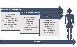
The exposome concept clearly illustrates the complexity of the environment humans are exposed to nowadays, and how this can impact human health. There is a need for internal biomarkers of exposure (see section on Human biomonitoring) as well as biomarkers of effect, to disentangle the complex interplay between several exposures occurring potentially simultaneously and at different concentrations throughout life. Advances in biomedical sciences and molecular biology thereby collecting holistic information of epigenetics, transcriptome (see section on Gene expression), metabolome (see section on Metabolomics), etc. are at the forefront to identify biomarkers of exposure as well as of effect.

Internal molecular markers of the exposome

Meet in the middlemodel

To determine the health effect of environmental exposure, markers that can detect early changes before disease arises are essential and can be implemented in preventative medicine. These types of markers can be seen as intermediate biomarkers of effect, and their discovery relies on large-scale studies at different levels of biology (transcriptomics, genomics, metabolomics). The term "omics" refers to the quantitative measurement of global sets of molecules in biological samples using high throughput techniques (i.e. automated experiments that enable large scale repetition)⁷, in combination with advanced biostatistics and bioinformatics tools⁸. Given the availability of data from high-throughput omics platforms, together with reliable measurements of external exposures, the use of omics enhances the search for markers playing a role in the biological pathway linking exposure to disease risk.

The meet-in-the-middle (MITM) concept was suggested as a way to address the challenge of identifying causal relationships linking exposures and disease outcome (Figure 2). The first step of this approach consists in the investigation of the association between exposure and biomarkers of exposure. The next step consists in the study of the relationship between (biomarkers of) exposure and intermediate omics biomarkers of early effects; and third, the relation between the disease outcome and intermediate omics biomarkers is assessed. The MITM stipulates that the causal nature of an association is reinforced if it is found in all three steps. Molecular markers that indicate susceptibility to certain environmental exposures are starting to become uncovered and can aid in targeted prevention strategies. Therefore, this approach is heavily dependent on new developments in molecular epidemiology, in which molecular biology is merged into epidemiological studies. Below, the different levels of molecular biology currently studied to identify markers of exposure and effect are discussed in detail.

Figure adapted from Vineis & Perera (2007).

Levels

Intermediate biomarkers can be identified as measurable indicators of certain biological states at different levels of the cellular machinery, and vary in their response time, duration, site and mechanism of action. Different molecular markers might be preferred depending on the exposure(s) under study.

Gene expression

Changes at the mRNA level can be studied following a candidate approach in which mRNAs with a biological role suspected to be involved in the molecular response to a certain type of exposure (e.g. inflammatory mRNAs in the case of exposure to tobacco smoke) are selected a priori and measured using quantitative PCR technology or alternatively at the level of the whole genome by means of microarray analyses or Next Generation Sequencing technology. ¹⁰ Changes at the transcriptome level, are studied by analysing the totality of RNA molecules present in a cell type or sample.

Both types of studies have proven their utility in molecular epidemiology. About a decade ago the first study was published reporting on candidate gene expression profiles that were associated with exposure to diverse carcinogens¹¹. Around the same time, the first studies on transcriptomics were published, including transcriptomic profiles for a dioxin-exposed population ¹², in association with diesel-exhaust exposure,¹³ and comparing smokers versus non-smokers both in blood ¹⁴ as well as airway epithelium cells¹⁵. More recently, attention has been focused on prenatal exposures in association with transcriptomic signatures, as this fits within the scope of the exposome concept. As such, transcriptomic profiles have been described in association with exposure to maternal smoking assessed in placental tissue,¹⁶ as well as particulate matter exposure in cord blood samples¹⁷.

Epigenetics

Epigenetics related to all heritable changes in that do not affect the DNA sequence itself directly. The most widely studied epigenetic mechanism in the field of environmental epidemiology to date is DNA methylation. DNA methylation refers to the process in which methyl-groups are added to a DNA sequence. As such, these methylation changes can alter the expression of a DNA segment without altering its sequence. DNA methylation can be studied by a candidate gene approach using a digestion-based design or, more commonly used, a bisulfite conversion followed by pyrosequencing, methylation-specific PCR or a bead array. The bisulfite treatment of DNA mediates the deamination of cytosine into uracil, and these converted residues will be read as thymine, as determined by PCR-amplification and sequencing. However, 5 mC residues are resistant to this conversion and will remain read as cytosine (Figure 3).

Figure 3: A. Restriction-digest based design A methylated (CH3) region of genomic DNA is digested either with two restriction enzymes, one which is blocked by GC methylation (HpaII) and one which is not(MspI). Smaller fragments are discarded (X), enriching for methylated DNA in the HpaII treated sample. B. Bisulfite-conversion of DNA. DNA is denatured and then treated with sodium bisulfite to convert unmethylated cytosine to uracil, which is converted to thymine by PCR. An important point is that following bisulfite conversion, the DNA strands are no longer complementary, and primers are designed to assay the methylation status of a specific strand.

If an untargeted approach is desirable, several strategies can be followed to obtain whole-genome methylation data, including sequencing. Epigenotyping technologies such as the human methylation BeadChips ¹⁸ generate a methylation-state-specific 'pseudo-SNP' through bisulfite conversion; therefore, translating differences in the DNA methylation patterns into sequence differences that can be analyzed using quantitative genotyping methods¹⁹.

An interesting characteristic of DNA methylation is that it can have transgenerational effects (i.e. effects that act across multiple generations). This was first shown in a study on a population that was prenatally exposed to famine during the Dutch Hunger Winter in 1944-1945. These individuals had less DNA methylation of the imprinted gene coding for insulin-like growth factor 2 (IGF2) measured 6 decades later compared with their unexposed, same-sex siblings. The association was specific for peri-conceptional exposure (i.e. exposure during the period from before conception to early pregnancy), reinforcing that very early mammalian development is a crucial period for establishing and maintaining epigenetic marks²⁰.

Post-translational modifications (i.e. referring to the biochemical modification of proteins following protein biosynthesis) recently gained more attention as they are known to be induced by oxidative stress ²¹ (see sections on Oxidative stress) and specific inflammatory mediators ²². Besides their function in the structure of chromatin in eukaryotic cells, histones have been shown to have toxic and pro-inflammatory activities when they are released into the extracellular space ²³. Much attention has gone to the associations between metal exposures and histone modifications,²⁴ although recently a first human study on the association between particulate matter exposure and histone H3 modification was published²⁵.

Expression of microRNAs (miRNAs are small noncoding RNAs of ∼22nt in length which are involved in the regulation of gene expression at the posttranscriptional level by degrading their target mRNAs and/or inhibiting their translation) {Ambros et al,2004}{Ambros, 2004 #324}{Ambros, 2004 #324} has also been shown to serve as a valuable marker of exposure, both candidate and untargeted approaches have resulted in the identification of miRNA expression patterns that are associated with exposure to smoking ²⁶, particulate matter ²⁷, and chemicals such as polychlorinated biphenyls (PCBs) ²⁸.

Metabolomics

Metabolomics have been proposed as a valuable approach to address the challenges of the exposome. Metabolomics, the study of metabolism at the whole-body level, involves assessment of the entire repertoire of small molecule metabolic products present in a biological sample. Unlike genes, transcripts and proteins, metabolites are not encoded in the genome. They are also chemically diverse, consisting of carbohydrates, amino acids, lipids, nucleotides and more. Humans are expected to contain a few thousand metabolites, including those they make themselves as well as nutrients and pollutants from their environment and substances produced by microbes in the gut. The study of metabolomics increases knowledge on the interactions between gene and protein expression, and the environment²⁹. Metabolomics can be a biomarker of effect of environmental exposure as it allows for the full characterization of biochemical changes that occur during xenobiotic metabolism (see Section on Xenobiotic metabolism and defence). Recent technological developments have allowed downscaling the sample volume necessary for the analysis of the full metabolome, allowing for the assessment of system-wide metabolic changes that occur as a result of an exposure or in conjunction with a health outcome ³⁰. As for all discussed biomarkers, both targeted metabolomics, in which specific metabolites are measured in order to characterize a pathway of interest, as well as untargeted metabolomic approaches are available. Among "omics" methodologies, metabolomics interrogates the levels of a relatively lower number of features as there are about 2900 known human metabolites versus ~30,000 genes. Therefore it has strong statistical power compared to transcriptome-wide and genome-wide studies ³¹. Metabolomics is, therefore, a potentially sensitive method for identifying biochemical effects of external stressors. Even though the developing field of "environmental metabolomics" seeks to employ metabolomic methodologies to characterize the effects of environmental exposures on organism function and health, the relationship between most of the chemicals and their effects on the human metabolome have not yet been studied.

Challenges

Limitations of molecular epidemiological studies include the difficulty to obtain samples to study, the need for large study populations to identify significant relations between exposure and the biomarker, the need for complex statistical methods to analyse the data. To circumvent the issue of sample collection, much effort has been focused on eliminating the need for blood or serum samples by utilizing saliva samples, buccal cells or nail clippings to read out molecular markers. Although these samples can be easily collected in a non-invasive manner, care must be taken to prove that these samples indeed accurately reflect the body's response to exposure rather than a local effect. For DNA methylation, it has been shown this is heavily dependent on the locus under study. For certain CpG sites the correlation in methylation levels is much higher than for other sites ³². For those sites that do not correlate well across tissues, it has furthermore been demonstrated that DNA methylation levels can differ in their associations with clinical outcomes ³³, so care must be taken in epidemiological study design to overcome these issues.

4.3.11. Question 6

Describe the 3 components of the exposome

---

4.3.11. Question 7

Explain how using the meet in the middle model biomarkers can be identified

---

4.3.11. Question 8

Give 3 examples of molecular (bio)markers of environmental exposure.

---

4.3.12. Gene expression

Author: Nico M. van Straalen

Reviewers: Dick Roelofs, Dave Spurgeon

Learning objectives:

You should be able to

• provide an overview of the various "omics" approaches (genomics, transcriptomics, proteomics and metabolomics) deployed in environmental toxicology.
• describe the practicalities of transcriptomics, how a transcription profile is generated and analysed.
• indicate the advantages and disadvantages of the use of genome-wide gene expression in environmental toxicology.
• develop an idea on how transcriptomics might be integrated into risk assessment of chemicals.

Keywords: genomics, transcriptomics, proteomics, metabolomics, risk assessment

Synopsis

Low-dose exposure to toxicants induces biochemical changes in an organism, which aim to maintain homoeostasis of the internal environment and to prevent damage. One aspect of these changes is a high abundance of transcripts of biotransformation enzymes, oxidative stress defence enzymes, heat shock proteins and many proteins related to the cellular stress response. Such defence mechanisms are often highly inducible, that is, their activity is greatly upregulated in response to a toxicant. It is also known that most of the stress responses are specific to the type of toxicant. This principle may be reversed: if an upregulated stress response is observed, this implies that the organism is exposed to a certain stress factor; the nature of the stress factor may even be derived from the transcription profile. For this reason, microarrays, RNA sequencing or other techniques of transcriptome analysis, have been applied in a large variety of contexts, both in laboratory experiments and in field surveys. These studies suggest that transcriptomics scores high on (in decreasing order) (1) rapidity, (2) specificity, and (3) sensitivity. While the promises of genomics applications in environmental toxicology are high, most of the applications are in mode-of-action studies rather than in risk assessment.

Introduction

No organism is defenceless against environmental toxicants. Even at exposures below phenotypically visible no-effect levels a host of physiological and biochemical defence mechanisms are already active and contribute to the organism's homeostasis. These regulatory mechanisms often involve upregulation of defence mechanisms such as oxidative stress defence, biotransformation (xenobiotic metabolism), heat shock responses, induction of metal-binding proteins, hypoxia response, repair of DNA damage, etc. At the same time downregulation is observed for energy metabolism and functions related to growth and reproduction. In addition to these targeted regulatory mechanisms targeting, there are usually a lot of secondary effects and dysfunctional changes arising from damage. A comprehensive overview of all these adjustments can be obtained from analysis of the transcriptome.

In this module we will review the various approaches adopted in "omics", with an emphasis on transcriptomics. "Omics" is a container term comprising five different activities. Table 1 provides a list of these approaches and their possible contribution to environmental toxicology. Genomics and transcriptomics deal with DNA and mRNA sequencing, proteomics relies on mass spectrometry while metabolomics involves a variety of separation and detection techniques, depending on the class of compounds analysed. The various approaches gain strength when applied jointly. For example proteomics analysis is much more insightful if it can be linked to an annotated genome sequence and metabolism studies can profit greatly from transcription profiles that include the enzymes responsible for metabolic reactions. Systems biology aims to integrate the different approaches using mathematical models. However, it is fair to say that the correlation between responses at the different levels is often rather poor. Upregulation of a transcript does not always imply more protein, more protein can be generated without transcriptional upregulation and the concentration of a metabolite is not always correlated with upregulation of the enzymes supposed to produce it. In this module we will focus on transcriptomics only. Metabolomics is dealt with in a separate section.

Table 1. Overview of the various "omics" approaches

Term	Description	Relevance for environmental toxicology
Genomics	Genome sequencing and assembly, comparison of genomes, phylogenetics, evolutionary analysis	Explanation of species and lineage differences in susceptibility from the structure of targets and metabolic potential, relationship between toxicology, evolution and ecology
Transcriptomics	Genome-wide transcriptome (mRNA) analysis, gene expression profiling	Target and metabolism expression indicating activity, analysis of modes of action, diagnosis of substance-specific effects, early warning instrument for risk assessment
Proteomics	Analysis of the protein complement of the cell or tissue	Systemic metabolism and detoxification, diagnosis of physiological status, long-term or permanent effects
Metabolomics	Analysis of all metabolites from a certain class, pathway analysis	Functional read-out of the physiological state of a cell or tissue
Systems biology	Integration of the various "omics" approaches, network analysis, modelling	Understanding of coherent responses, extrapolation to whole-body phenotypic responses

Transcriptomics analysis

The aim of transcriptomics in environmental toxicology is to gain a complete overview of all changes in mRNA abundance in a cell or tissue as a function of exposure to environmental chemicals. This is usually done in the following sequence of steps:

1. Exposure of organisms to an environmental toxicant, including a range of concentrations, time-points, etc., depending on the objectives of the experiment.
2. Isolation of total RNA from individuals or a sample of pooled individuals. The number of biological replicates is determined at this stage, by the number of independent RNA isolations, not by technical replication further on in the procedure.
3. Reverse transcription. mRNAs are transcribed to cDNA using the enzyme reverse transcriptase that initiates at the polyA tail of mRNAs. Because ribosomal RNA lacks a poly(A)tail they are (in principle) not transcribed to cDNA. This is followed by size selection and sometimes labelling of cDNAs with barcodes to facilitate sequencing.
4. Sequencing of the cDNA pool and transcriptome assembly. The assembly preferably makes use of a reference genome for the species.If no reference genome is available, the transcriptome is assembled de novo, which requires a greater sequencing depth and usually ends in many incomplete transcripts. A variety of corrections are applied to equalize effects of total RNA yield, library size, sequencing depth, gene length, etc.
5. Gene expression analysis and estimation of fold regulation. This is done, in principle, by counting the normalized number of transcripts per gene for every gene in the genome, for each of the different conditions to which the organism was exposed. The response per gene is expressed as fold regulation, by expressing the transcripts relative to a standard or control condition. Tests are conducted to separate significant changes from noise.
6. Annotation and assessment of pathways and functions as influenced by exposure. An integrative picture is developed, taking all evidence together, of the functional changes in the organism.

In the recent past, step 4 was done by microarray hybridization rather than by direct sequencing. In this technique two pools of cDNA (e.g. a control and a treatment) are hybridized to a large number of probes fixed onto a small glass plate. The probes are designed to represent the complete gene complement of the organism. Positive hybridization signals are taken as evidence for upregulated gene expression. Microarray hybridization arose in the years 1995-2005 but has now been largely overtaken by ultrafast and high-throughput next generation sequencing methods, however, due to cost-efficiency, relative simplicity of bioinformatics analysis, and standardization of the assessed genes it is still often used.

We illustrate the principles of transcriptomics analysis and the kind of data analysis that follows it, by an example from the work by Bundy et al. (2008). These authors exposed earthworms (Lumbricus rubellus) to soils experimentally amended with copper, quite a toxic element for earthworms. The copper-induced transcriptome was surveyed using a custom-made microarray and metabolic profiles were established using NMR (nuclear magnetic resonance) spectroscopy. From the 8,209 probes on the microarray, 329 showed a significant alteration of expression under the influence of copper. The data were plotted in a "heat map" diagram (Figures 1A and 1B), providing a quick overview of upregulated and downregulated genes. The expression profiles were also analysed in reduced dimensionality using principal component analysis (PCA). This showed that the profiles varied considerably with treatment. Especially the highest and the penultimate highest exposures generated a profile very different from the control (see Figure 1C). The genes could be allocated to four clusters, (1) genes upregulated by copper over all exposures (Figure 1D), (2) genes downregulated by copper (see Figure 1E), (3) genes upregulated by low exposures but unaffected at higher exposures (see Figure 1F), and (4) genes upregulated by low exposure but downregulated by higher concentrations (see Figure 1G). Analysis of gene identity combined with metabolite analysis suggested that the changes were due to an effect of copper on mitochondrial respiration, reducing the amount of energy generated by oxidative phosphorylation. This mechanism was underlying the reduction of body-growth observed on the phenotypic level.

Figure 1. Example of a transcriptomics analysis aiming to understand copper toxicity to earthworms. A "heat map" of individual replicates (four in each of five copper treatments). Expression is indicated for each of the 329 differentially expressed genes (arranged from top to bottom) in red (downregulated) or green (upregulated). A cluster analysis showing the similarities is indicated above the profiles. B. The same data, but with the four replicates per copper treatment joined. The data show that at 40 mg/kg of copper in soil some of the earthworm's genes are starting to be downregulated, while at 160 mg/kg and 480 mg/kg significant upregulation and downregulation is occurring. C Principal Component Analysis of the changes in expression profile. The multivariate expression profile is reduced to two dimensions and the position of each replicate is indicated by a single point in the biplot; the confidence interval over four replicates of each copper treatment is indicated by horizontal and vertical bars. The profiles of the different copper treatments (joined by a dashed line) differ significantly from each other. D, E, F, and G. Classification of the 329 genes in four groups according to their responses to copper (plotted on the horizontal axis). Redrawn from Bundy et al. (2008) by Wilma Ijzerman.

Omics in risk assessment

How could omics-technology, especially transcriptomics, contribute to risk assessment of chemicals? Three possible advantages have been put forward:

1. Gene expression analysis is rapid. Gene regulation takes place on a time-scale of hours and results can be obtained within a few days. This compares very favourably with traditional toxicity testing (Daphnia, 48 hours, Folsomia, 28 days).
2. Gene expression is specific. Because a transcription profile involves hundreds to thousands of endpoints (genes), the information content is potentially very large. By comparing a new profile generated by an unknown compound, to a trained data set, the compound can usually be identified quite precisely.
3. Gene expression is sensitive. Because gene regulation is among the very first biochemical responses in an organism, it is expected to respond to lower dosages, at which whole-body parameters such as survival, growth and reproduction are not yet responding.

Among these advantages, the second one (specificity) has shown to be the most consistent and possibly brings the largest advantage. This can be illustrated by a study by Dom et al. (2012) in which gene expression profiles were generated for Daphnia magna exposed to different alcohols and chlorinated anilines (Figure 2).

Figure 2. Clustered gene expression profiles of Daphnia magna exposed to seven different compounds. Replicates exposed to the same compound are clustered together, except for ethanol. The first split separates exposures that at the EC10 level (reproduction) did not show any effects on growth and energy reserves (right) and exposures that caused significant such effects (left). Reproduced from Dom et al. (2012) by Wilma IJzerman.

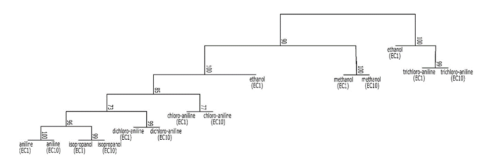
The profiles of replicates exposed to the same compound were always clustered together, except in one case (ethanol), showing that gene expression is quite specific to the compound. It is possible to reverse this argument: from the gene expression profile the compound causing it can be deduced. In addition, the example cited showed that the first separation in the cluster analysis was between exposures that did and did not affect energy reserves and growth. So the gene expression profiles are not only indicative of the compound, but also of the type of effects expected.

The claim of rapidity also proved true, however, the advantage of rapidity is not always borne out. It may be an issue when quick decisions are crucial (evaluating a truck loaded with suspect contaminated soil, deciding whether to discharge a certain waste stream into a lake yes or no), but for regular risk assessment procedures it proved to be less of an advantage than sometimes expected. Finally, greater sensitivity of gene expression, in the sense of lower no-observed effect concentrations than classical endpoints is a potential advantage, but proves to be less spectacular in practice. However, there are clear examples in which exposures below phenotypic effect levels were shown to induce gene expression responses, indicating that the organism was able to compensate any negative effects by adjusting its biochemistry.

Another strategy regarding the use of gene expression in risk assessment is not to focus on genome-wide transcriptomes but on selected biomarker genes. In this strategy, gene expressions are aimed for that show (1) consistent dose-dependency, (2) responses over a wide range of contaminants, and (3) correlations with biological damage. For example, De Boer et al. (2015) analysed a composite data set including experiments with six heavy metals, six chlorinated anilines, tetrachlorobenzene, phenanthrene, diclofenac and isothiocyanate, all previously used in standardized experiments with the soil-living collembolan, Folsomia candida. Across all treatments a selection of 61 genes was made, that were responsive in all cases and fulfilled the three criteria listed above. Some of these marker genes showed a very good and reproducible dose-related response to soil contamination. Two biomarkers are shown in Figure 3. This experiment, designed to diagnose a field soil with complex unknown contamination, clearly demonstrated the presence of Cyp-inducing organic toxicants.

Figure 3. Showing gene expression, relative to control expression, for two selected biomarker genes (encoding cytochroms P450 phase I biotransformation enzymes) in the genome of the soil-living collembolan Folsomia candida, in response to the concentration of contaminated field soil spiked-in into a clean soil at different rates. Reproduced from Roelofs et al. (2012) by Wilma IJzerman.

Of course there are also disadvantages associated with transcriptomics in environmental toxicology, for example:

1. Gene expression analysis requires a knowledge-intensive infrastructure, including a high level of expertise for some of the bioinformatics analyses. Also, adequate molecular laboratory facilities are needed; some techniques are quite expensive.
2. Gene expression analysis is most fruitful when species are used that are backed up by adequate genomic resources, especially a well annotated genome assembly, although this is becoming less of a problem with increasing availability of genomic resources.
3. The relationship between gene expression and ecologically relevant variables such as growth and reproduction of the animal is not always clear.

Conclusions

Gene expression analysis has come to occupy a designated niche in environmental toxicology since about 2005. It is a field highly driven by technology, and shows continuous change over the last years. It may significantly contribute to risk assessment in the context of mode of action studies and as a source of designated biomarker techniques. Finally, transcriptomics data are very suitable to feed into information regarding key events, important biochemical alterations that are causally linked up to the level of the phenotype to form an adverse outcome pathway. We refer to the section on Adverse outcome pathways for further reading.

References

Bundy, J.G., Sidhu, J.K., Rana, F., Spurgeon, D.J., Svendsen, C., Wren, J.F., Stürzenbaum, S.R., Morgan, A.J., Kille, P. (2008). "Systems toxicology" approach identifies coordinated metabolic responses to copper in a terrestrial non-model invertebrate, the earthworm Lumbricus rubellus. BMC Biology 6, 25.

De Boer, T.E., Janssens, T.K.S., Legler, J., Van Straalen, N.M., Roelofs, D. (2015). Combined transcriptomics analysis for classification of adverse effects as a potential end point in effect based screening. Environmental Science and Technology 49, 14274-14281.

Dom, N., Vergauwen, L., Vandenbrouck, T., Jansen, M., Blust, R., Knapen, D. (2012). Physiological and molecular effect assessment versus physico-chemistry based mode of action schemes: Daphnia magna exposed to narcotics and polar narcotics. Environmental Science and Technology 46, 10-18.

Gibson, G., Muse, S.V. (2002). A Primer of Genome Science. Sinauer Associates Inc., Sunderland.

Gibson, G. (2008). The environmental contribution to gene expression profiles. Nature Reviews Genetics 9, 575-581.

Roelofs, D., De Boer, M., Agamennone, V., Bouchier, P., Legler, J., Van Straalen, N. (2012). Functional environmental genomics of a municipal landfill soil. Frontiers in Genetics 3, 85.

Van Straalen, N.M., Feder, M.E. (2012). Ecological and evolutionary functional genomics - how can it contribute to the risk assessment of chemicals? Environmental Science & Technology 46, 3-9.

Van Straalen, N.M., Roelofs, D. (2008). Genomics technology for assessing soil pollution. Journal of Biology 7, 19.

4.3.12. Question 1

Define: (1) genomics, (2) transcriptomics (3) proteomics, and (4) metabolomics, and indicate which of these approaches is most useful in the risk assessment of chemicals.

---

4.3.12. Question 2

Specify three advantages and at least one disadvantage of the use of genome-wide gene expression as a tool in environmental risk assessment.

---

4.3.13. Metabolomics

Author: Pim E.G. Leonards

Reviewers: Nico van Straalen, Drew Ekman

Learning objectives:

You should be able to:

• understands the basics of metabolomics and how metabolomics can be used.
• describe the basic principles of metabolomics analysis, and how a metabolic profile is generated and analysed.
• describe the differences between targeted and untargeted metabolomics and how each is used in environmental toxicology.
• develop an idea on how metabolomics might be integrated into hazard and risk assessments of chemicals.

Keywords: Metabolomics, metabolome, environmental metabolomics, application areas of metabolomics, targeted and untargeted metabolomics, metabolomics analysis and workflow

Introduction

Metabolomics is the systematic study of small organic molecules (<1000 Da) that are intermediates and products formed in cells and biofluids due to metabolic processes. A great variety of small molecules result from the interaction between genes, proteins and metabolites. The primary types of small organic molecules studied are endogenous metabolites (i.e., those that occur naturally in the cell) such as sugars, amino acids, neurotransmitters, hormones, vitamins, and fatty acids. The total number of endogenous metabolites in an organism is still under study but is estimated to be in the thousands. However, this number varies considerably between species and cell types. For instance, brain cells contain relative high levels of neurotransmitters and lipids, nevertheless the levels between different types of brain tissues can vary largely. Metabolites are working in a network, e.g. citric acid cycle, by the conversion of molecules by enzymes. The turnover time of the metabolites is regulated by the enzymes present and the amount of metabolites present.

The field of metabolomics is relatively new compared to genomics, with the first draft of the human metabolome available in 2007. However, the field has grown rapidly since that time due to its recognized ability to reflect molecular changes most closely associated with an organism's phenotype. Indeed, in comparison to other 'omics approaches (e.g., transcriptomics), metabolites are the downstream results from the action of genes and proteins and, as such, provide a direct link with the phenotype (Figure 1). The metabolic status of an organism is directly related to its function (e.g. energetic, oxidative, endocrine, and reproductive status) and phenotype, and is, therefore, uniquely suitable to relate chemical stress to the health status of organisms. Moreover, transcriptomics and proteomics, the identification of metabolites does not require the existence of gene sequences, making it particularly useful for the those species which lack a sequenced genome.

Figure 1: Cascade of different omics fields.

Definitions

The complete set of small molecules in a biological system (e.g. cells, body fluids, tissues, organism) is called the metabolome (Table 1). The term metabolomics was introduced by Oliver et al. (1998) who described it "as the complete set of metabolites/low molecular weight compounds which is context dependent, varying according to the physiology, development or pathological state of the cell, tissue, organ or organism". This quote highlights the observation that the levels of metabolites can vary due to internal as well as external factors, including stress resulting from exposure to environmental contaminants. This has resulted in the emergence and growth of the field of environmental metabolomics which is based on the application of metabolomics, to biological systems that are exposed to environmental contaminants and other relevant stressors (e.g., temperature). In addition to endogenous metabolites, some metabolomic studies also measure changes in the biotransformation of environmental contaminants, food additives, or drugs in cells, the collection of which has been termed the xenometabolome.

Table 1: Definitions of metabolomics.

Term	Definition	Relevance for environmental toxicology
Metabolomics	Analysis of small organic molecules (<1000 Da) in biological systems (e.g. cell, tissue, organism)	Functional read-out of the physiological state of a cell or tissue and directly related to the phenotype
Metabolome	Measurement of the complete set of small molecules in a biological system	Discovery of affected metabolic pathways due to contaminant exposure
Environmental metabolomics	Metabolomics analysis in biological systems that are exposed to environmental stress, such as the exposure to environmental contaminants	Metabolomics focused on environmental contaminant exposure to study for instance the mechanism of toxicity or to find a biomarker of exposure or effect
Xenometabolome	Metabolites formed from the biotransformation of environmental contaminants, food additives, or drugs	Understanding the metabolism of the target contaminant
Targeted metabolomics	Analysis of a pre-selected set of metabolites in a biological system	Focus on the effects of environmental contaminants on specific metabolic pathways
Untargeted metabolomics	Analysis of all detectable (i.e., not preselected) of metabolites in a biological system	Discovery-based analysis of the metabolic pathways affected by environmental contaminant exposure

Environmental Metabolomics Analysis

The development and successful application of metabolomics relies heavily on i) currently available analytical techniques that measure metabolites in cells, tissues, and organisms, ii) the identification of the chemical structures of the metabolites, and iii) characterisation of the metabolic variability within cells, tissues, and organisms.

The aim of metabolomics analysis in environmental toxicology can be:

• to focus on changes in the abundances of specific metabolites in a biological system

after environmental contaminant exposure: targeted metabolomics

• to provide a "complete" overview of changes in abundances of all detectable metabolites in a biological system after environmental contaminant exposure: untargeted metabolomics

In targeted metabolomics a limited number of pre-selected metabolites (typically 1-100) are quantitatively analysed (e.g. nmol dopamine/g tissue). For example, metabolites in the neurotransmitter biosynthetic pathway could be targeted to assess exposures to pesticides. Targeting specific metabolites in this way typically allows for their detection at low concentrations with high accuracy. Conversely, in untargeted metabolomics the aim is to detect as many metabolites as possible, regardless of their identities so as to assess as much of the metabolome as possible. The largest challenge for untargeted metabolomics is the identification (annotation) of the chemical structures of the detected metabolites. There is currently no single analytical method able to detect all metabolites in a sample, and therefore a combination of different analytical techniques are used to detect the metabolome. Different techniques are required due to the wide range of physical-chemical properties of the metabolites. The variety of chemical structures of metabolites are shown in Figure 2. Metabolites can be grouped in classes such as fatty acids (the classes are given in brackets in Figure 2), and within a class different metabolites can be found.

Figure 2: Examples of the chemical structures of several commonly detected metabolites. Metabolite classes are indicated in brackets. Drawn by Steven Droge.

A general workflow of environmental metabolomics analysis uses the following steps:

1. of the organism or cells to an environmental contaminant. An unexposed control group must also be included. The exposures often include the use of various concentrations, time-points, etc., depending on the objectives of the study.
2. Sample collection of the relevant biological material (e.g. cell, tissue, organism). It is important that the collection be done as quickly as possible so as to quench any further metabolism. Typically ice cold solvents are used.
3. of the metabolites from the cell, tissue or organisms by a two-step extraction using a combination of polar (e.g. water/methanol) and apolar (e.g. chloroform) extraction solvents.
4. of the polar and apolar fractions using liquid chromatography (LC) or gas chromatography (GC) combined with mass spectrometry (MS), or by nuclear magnetic resonance (NMR) spectroscopy. The analytical tool(s) used will depend on the metabolites under consideration and whether a targeted or untargeted approach is required.
5. Metabolite detection (targeted or untargeted analysis).
   • Targeted metabolomics - a specific set of pre-selected metabolites are detectedand their concentrations are determined using authentic standards.
   • Untargeted metabolomics - a list of all detectable metabolites measured by MS or NMR response, and their intensities is collected. Various techniques are then used to determine the identities of those metabolites that change due to the exposure (see step 7 below).
6. Statistical analysis using univariate and multivariate statistics to calculate the difference between the exposure and the control groups. The fold change (fold increase or decrease of the metabolite levels) between an exposure and control group are determined.
7. For untargeted metabolomics only the chemical structure of the statistically significant metabolites are identified. The identification of the chemical structure of the metabolite can be based on the molecular weight, isotope patterns, elemental compositions, mass spectrometry fragmentation patterns, etc. Mass spectrometry libraries are used for the identification to match the above parameters in the samples with the data in libraries.
8. Data processing: Identification of the metabolic pathways influenced by the chemical exposure. Integrative picture of the molecular and functional level of an organism due to chemical exposure. Understand the relationship between the chemical exposure, molecular pathway changes and the observed toxicity. Or to identify potential biomarkers of exposure or effect.

Box: Analytical tools for metabolomics analysis The most frequently used analytical tools for measuring metabolites are mass spectrometry (MS) and nuclear magnetic resonance (NMR) spectroscopy. MS is an analytical tool that generates ions of molecules and then measures their mass-to-charge ratios. This information can be used to generate a "molecular finger print" for each molecule, and based on this finger print metabolites can be identified. Chromatography is typically used to separate the different metabolites of a mixture found in a sample before it enters the mass spectrometer. Two main chromatography techniques are used in metabolomics: liquid chromatography and gas chromatography. Due to its high sensitivity, MS is able to measure a large number of different metabolites simultaneously. Moreover, when coupled with a separation method such as chromatography, MS can detect and identify thousands of metabolites. Mass spectrometry is much more sensitive than NMR, and it can detect a large range of different types of metabolites with different physical-chemical properties. NMR is less sensitive and can therefore detect a lower number of metabolites (typically 50-200). The advantages of NMR are the minimum amount of sample handling, the reproducibility of the measurements (due to high precision), and it is easier to quantify the levels of metabolites. In addition, NMR is a non-destructive technique such that a sample can often be used for further analyses after the data has been acquired.

Application of environmental metabolomics

Metabolomics has been widely used in drug discovery and medical sciences. More recently, metabolomics is being incorporated into environmental studies, an emerging field of research called environmental metabolomics. Environmental metabolomics is used mainly in five application domains (Table 2). Arguably the most commonly used application is for studying the mechanism of toxicity/mode of action (MoA) of contaminants. However, many studies have identified select metabolites that show promise for use as biomarkers of exposure or effect. As a result of its strength in identifying response fingerprints, metabolomics is also finding use in the regulatory toxicology field particularly for read-across studies. This application is particularly useful for rapidly screening contaminants for toxicity. Metabolomics can be also be used in dose-response studies (benchmark dosing) to derive a point of departure (POD). This is especially interesting in regulatory chemical risk assessment.

Currently, the field of systems toxicology is explored by combining data from different omics field (e.g. transcriptomics, proteomics, metabolomics) to improve our understanding of the relationship between the different omics, chemical exposure, and toxicity, and to better understand the mechanism of toxicity/ MoA.

Table 2: Application areas of metabolomics in environmental toxicology.

Application area	Description
Mechanism of toxicity/ Mode of action (MoA)	Using metabolomics to understand at the molecular level the pathways that are affected by exposure to environmental contaminants. Discovery of the mode of action of chemicals. In an adverse outcome pathway (AOP)Discovery metabolomics is used to identify the key events (KE), by linking chemical exposure at the molecular level to functional endpoints (e.g. reproduction, behaviour).
Biomarker discovery	Identification of metabolites that can be used as convenient (i.e., easy and inexpensive to measure) indicators of exposure or effect.
Read-across	In regulatory toxicology, metabolomics is used in read-across studies to provide information on the similarity of the responses between chemicals. This approach is useful to identify more environmentally toxic chemicals.
Point of departure	Metabolomics can be used in dose-response studies (benchmark dosing) to derive a point of departure (POD). This is especially interesting in regulatory chemical risk assessment. This application is currently not used yet.
Systems toxicology	Combination approach of different omics (e.g. transcriptomics, proteomics, metabolomics) to improve our understanding of the relationship between the different omics and chemical exposure, and to better understand the mechanism of toxicity/ MoA.

As an illustration of the mechanism of toxicity/mode of action application, Bundy et al. (2008) used NMR-based metabolomics to study earthworms (Lumbricus rubellus) exposed to various concentrations of copper in soil (0, 10, 40, 160, 480 mg copper / kg soil). They performed both transcriptomic and metabolomics studies. Both polar (sugars, amino acid, etc.) and apolar (lipids) metabolites were analysed, and fold changes relative to the control group were determined. For example, differences in the fold changes of lipid metabolites (e.g. fatty acids, triacylglycerol) as a function of copper concentration are shown as a "heatmap" in Figure 3A. Clearly the highest dose group (480 mg/kg) has a very different lipid metabolite pattern than the other groups. The polar metabolite data was analysed using principal component analysis (PCA) , a multivariate statistical tool that reduces the number of dimensions of the data. The PCA score plot shown in Figure 3B reveals that the largest differences in metabolite profiles exist between: the control and low dose (10 mg Cu/kg) groups, the 40 mg Cu/kg and 160 mg Cu/kg groups, and the highest dose (480 mg Cu/kg) group (Figure 3B). These separations indicate that the metabolite patterns in these groups were different as a result of the different copper exposures. Some of the metabolites were up- and some were down-regulated due to the copper exposure (two examples given in Figures 3c and 3D). The metabolite data were also combined with gene expression data in a systems toxicology application. This combined analysis showed that the copper exposures led to disruption of energy metabolism, particularly with regard to effects on the mitochondria and oxidative phosphorylation. Bundy et al. associated this effect on energy metabolism with a reduced growth rate of the earthworms. This study effectively showed that metabolomics can be used to understand the metabolite pathways that are affected by copper exposure and are closely linked to phenotypic changes (i.e., reduced growth rate). The transcriptome data collected simultaneously were in good accordance with the metabolome patterns, supporting Bundy et al.'s hypothesis that simultaneous measurement of the transcriptomes and metabolome can be used to validate the findings of both approaches, and in turn the value of "systems toxicology".

Figure 3: Example of metabolite analysis with NMR to understand the mechanism of toxicity of copper to earthworms (Bundy et al., 2008). A: Heatmap, showing the fold changes of lipid metabolites at different exposure concentrations of copper (10, 40, 160, 480 mg/kg copper in soil) and controls. B: Principal component analysis (PCA) of the polar metabolite patterns of the exposure groups. The higher dose group (480 mg/kg soil) is separate from the medium dose (40 mg Cu/kg and 160 mg Cu/kg) groups and the control and the lowest dose groups (0 mg Cu/kg and 10 mg Cu/kg soil) indicating that the metabolite patterns in these groups are different and are affected by the copper exposure. C: Down and upregulation of lipophilic amino acids (blue: aliphatics, red: aromatics). D: Upregulation of cell-membrane-related metabolites (black = betaine, glycine, HEFS, phosphoethanolamine, red: myo-inositol, scyllo-inositol). Redrawn from Bundy et al. (2008) by Wilma IJzerman.

Challenges in metabolomics

Several challenges currently exist in the field of metabolomics. From a biological perspective, metabolism is a dynamic process and therefore very time-sensitive. Taking samples at different time-points during development of an organism, or throughout a chemical exposure can result in quite different metabolite patterns. Sample handling and storage can also be challenging as some metabolites are very unstable during sample collection and sample treatment. From an analytical perspective, metabolites possess a wide range of physico-chemical properties and occur in highly varying concentrations such that capturing the widest portion of the metabolome requires analysis with more than one analytical technique. However, the largest challenge is arguably the identification of the chemical structure of unknown metabolites. Even with state-of-the-art analytical techniques only a fraction of the unknown metabolites can be confidently identified.

Conclusions

Metabolomics is a relative new field in toxicology, but is rapidly increasing our understanding of the biochemical pathways affected by exposure to environmental contaminants, and in turn their mechanisms of action. Linking the changed molecular pathways due to the contaminant exposure to phenotypical changes of the organisms is an area of great interest. Continual advances in state-of-the-art analytical tools for metabolite detection and identification will continue to this trend and expand the utility of environmental metabolomics for prioritizing contaminants. However, a number of challenges remain for the widespread use of metabolomics in regulatory toxicology. Fortunately, recent growth in international interest to address these challenges is underway, and is making great strides in a variety of applications.

References

Bundy, J.G., Sidhu, J.K., Rana, F., Spurgeon, D.J., Svendsen, C., Wren, J.F., Sturzenbaum, S.R., Morgan, A.J., Kille, P. (2008). 'Systems toxicology' approach identifies coordinated metabolic responses to copper in a terrestrial non-model invertebrate, the earthworm Lumbricus rubellus. BMC Biology, 6(25), 1-21.

Bundy, J.G., Matthew P. Davey, M.P., Viant, M.R. (2009). Environmental metabolomics: a critical review and future perspectives. Metabolomics, 5, 3-21.

Johnson, C.H., Ivanisevic, J., Siuzdak, G. (2016). Metabolomics: beyond biomarkers and towards mechanisms. Nature Reviews, Molecular and Cellular Biology 17, 451-459.

4.3.13. Question 1

What type of molecules are measured with metabolomics?

Proteins

Small molecules

Genes

Polymers

---

4.3.13. Question 2

What are typical application areas of environmental metabolomics?

---

4.3.13. Question 3

Give four main elements of the workflow of metabolomics, and describe two in more detail?

---