4.1: Toxicokinetics

Last updated
Save as PDF

Page ID: 294554

Sylvia Moes, Kees van Gestel, & Gerco van Beek

\( \newcommand{\vecs}[1]{\overset { \scriptstyle \rightharpoonup} {\mathbf{#1}} } \) \( \newcommand{\vecd}[1]{\overset{-\!-\!\rightharpoonup}{\vphantom{a}\smash {#1}}} \)\(\newcommand{\id}{\mathrm{id}}\) \( \newcommand{\Span}{\mathrm{span}}\) \( \newcommand{\kernel}{\mathrm{null}\,}\) \( \newcommand{\range}{\mathrm{range}\,}\) \( \newcommand{\RealPart}{\mathrm{Re}}\) \( \newcommand{\ImaginaryPart}{\mathrm{Im}}\) \( \newcommand{\Argument}{\mathrm{Arg}}\) \( \newcommand{\norm}[1]{\| #1 \|}\) \( \newcommand{\inner}[2]{\langle #1, #2 \rangle}\) \( \newcommand{\Span}{\mathrm{span}}\) \(\newcommand{\id}{\mathrm{id}}\) \( \newcommand{\Span}{\mathrm{span}}\) \( \newcommand{\kernel}{\mathrm{null}\,}\) \( \newcommand{\range}{\mathrm{range}\,}\) \( \newcommand{\RealPart}{\mathrm{Re}}\) \( \newcommand{\ImaginaryPart}{\mathrm{Im}}\) \( \newcommand{\Argument}{\mathrm{Arg}}\) \( \newcommand{\norm}[1]{\| #1 \|}\) \( \newcommand{\inner}[2]{\langle #1, #2 \rangle}\) \( \newcommand{\Span}{\mathrm{span}}\)\(\newcommand{\AA}{\unicode[.8,0]{x212B}}\)

4.1. Toxicokinetics

Author: Nico van Straalen

Reviewer: Kees van Gestel

Learning objectives:

You should be able to

Describe the difference between toxicokinetics and toxicodynamics
Explain the use of different descriptors for the uptake of chemicals by organisms under steady state and dynamic conditions

Keywords: toxicodynamics, toxicokinetics, bioaccumulation, toxicokinetic rate constants, critical body residue, detoxification

Toxicology usually distinguishes between toxicokinetics and toxicodynamics. Toxicokinetics involves all processes related to uptake, internal transport and the accumulation inside an organism, while toxicodynamics deals with the interaction of a compound with a receptor, induction of defence mechanisms, damage repair and toxic effects. Of course the two sets of processes may interact, for instance defence may feed-back to uptake and damage may change the internal transport. However, often toxicokinetics analysis just focuses on tracking of the chemical itself and ignores possible toxic effects. This holds up to a critical threshold, the critical body concentration, above which effects become obvious and the normal toxicokinetics analysis is no longer valid. The assumption that toxicokinetic rate parameters are independent of the internal concentration is due the limited amount of information that can be obtained from animals in the environment. However, in so called physiology-based pharmacokinetic and pharmacodynamic models (PBPK models) kinetics and dynamics are analyzed as an integrated whole. The use of such models is however mostly limited to mammals and humans.

It must be emphasized that toxicokinetics considers fluxes and rates, i.e. mg of a substance moving per time unit from one compartment to another. Fluxes may lead to a dynamic equilibrium, i.e. an equilibrium that is due to inflow being equal to outflow; when only the equilibrium conditions are considered, this is called partitioning.

In this Chapter 4.1 we will explore the various approaches in toxicokinetics, including the fluxes of toxicants through individual organisms and through trophic levels as well as the biological processes that determine such fluxes. We start by comparing the concentrations of toxicants between organisms and their environment (section 4.1.1), and between organisms of different trophic levels (section 4.1.6). This leads to the famous concept of bioaccumulation, one of the properties of a substance often leading to environmental problems. While in the past dilution was sometimes seen as a solution to pollution, this is not correct for bioaccumulating substances, since they may turn up elsewhere in the next level food-chain and reach an even higher concentration. The bioaccumulation factor is one of the best-investigated properties characterizing the environmental behaviour of a substance . It may be predicted from properties of the substance such as the octanol-water partitioning coefficient.

In section 4.1.2 we discuss the classical theory of uptake-elimination kinetics using the one-compartment linear model. This theory is a crucial part of toxicological analysis. One of the first things you want to know about a substance is how quickly it enters an organism and how quickly it is removed. Since toxicity is basically a time-dependent process, the turnover rate of the internal concentration and the build-up of a residue depend upon the exposure time. An understanding of toxicokinetics is therefore critical to any interpretation of a toxicity experiment. Rate parameters may partly be predicted from substance properties, but properties of the organism play a much greater role here. One of these is simply the body mass; prediction of elimination rate constants from body mass is done by allometric scaling relationships, explored in section 4.1.5.

In two sections, 4.1.3 and 4.1.4, we present the biological processes that underlie the turnover of toxicants in an organism. These are very different for metals than for organic substances, hence, two separate sections are devoted to this topic, one on tissue accumulation of metals and one on defence mechanisms for organic xenobiotics.

Finally, if we understand all toxicokinetic processes we will also be able to understand whether the concentration inside a target organ will stay below or just passes the threshold that can be tolerated. The critical body concentration, explored in section 4.1.7 is an important concept linking toxicokinetics to toxicity.

4.1. Question 1

Define and indicate the differences between

Toxicokinetics
Toxicodynamics
Partitioning
Accumulation
Bioaccumulation

4.1.1. Bioaccumulation

Author: Joop Hermens

Reviewers: Kees van Gestel and Philipp Mayer

Learning objectives:

You should be able to

define and explain different bioaccumulation parameters.
Mention different biological factors that may affect bioaccumulation.

Key words: Bioaccumulation, lipid content

Introduction: terminology for bioaccumulation

The term bioaccumulation describes the transfer and accumulation of a chemical from the environment into an organism." For a chemical like hexachlorobenzene, the concentration in fish is more than 10,000 times higher than in water, which is a clear illustration of "bioaccumulation". A chemical like hexachlorobenzene is hydrophobic, so has a very low aqueous solubility. It therefore prefers to escape the aqueous phase to enter (or partition into) a more lipophilic phase such as the lipid phase in biota.

Uptake may take place from different sources. Fish mostly take up chemicals from the aqueous phase, organisms living at the sediment-water interphase are exposed via the overlying water and sediment particles, organisms living in soil or sediment via pore water and by ingesting soil or sediment, while predators will be exposed via their food. In many cases, uptake is related to more than one source. The different uptake routes are also reflected in the parameters and terminology used in bioaccumulation studies. The different parameters include the bioconcentration factor (BCF), bioaccumulation factor (BAF), biomagnification factor (BMF) and biota-to-sediment or biota-to-soil accumulation factor (BSAF). Figure 1 summarizes the definition of these parameters. Bioconcentration refers to uptake from the aqueous phase, bioaccumulation to uptake via both the aqueous phase and the ingestion of sediment or soil particles, while biomagnification expresses the accumulation of contaminants from food.

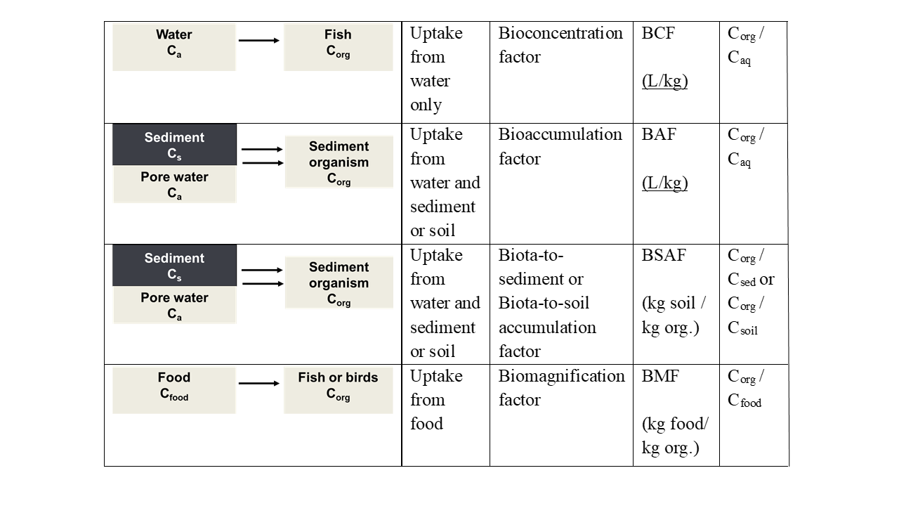
alt — Figure 1. Parameters used to describe the bioaccumulation of chemicals.

C_aq concentration in water (aqueous phase)

C_org concentration in organism

C_f concentration in food

C_s concentration in sediment or soil

Please note that the bioaccumulation factor (BAF) is defined in a similar way as the bioconcentration Factor (BCF), but that uptake can be both from the aqueous phase and the sediment or soil and that the exposure concentration usually is expressed per kg dry sediment or soil. Other definitions of the BAF are possible, but we have followed the one from Mackay et al. (2013). "The bioaccumulation factor (BAF) is defined here in a similar fashion as the BCF; in other words, BAF is CF/CW at steady state, except that in this case the fish is exposed to both water and food; thus, an additional input of chemical from dietary assimilation takes place".

All bioaccumulation factors are steady state constants: the concentration in the organism constant and the organisms is in equilibrium with its surrounding phase. It will take time before such an steady state is reached. Steady state is reached when uptake rate (for example from an aqueous phase) equals the elimination rate. Models that include the factor time in describing the uptake are called kinetic models; see section on Bioaccumulation kinetics.

Effect of biological properties on accumulation

Uptake of chemicals is determined by properties of both the organism and the chemical. For xenobiotic lipophilic chemicals in water, organism-specific factors usually play a minor role and concentrations in organisms can pretty well be predicted from chemical properties (see section on Structure-property relationships). For metals, on the contrary, uptake is to a large extent determined by properties of the organism, and a direct consequence of its mineral requirements. A chemical with low bioavailability (low uptake compared to concentration in exposure medium) may nevertheless accumulate to high levels when the organism is not capable of excreting or metabolising the chemical.

Factors related to the organism are:

Fat content. Because lipophilic chemicals mainly accumulate in the fat of organisms, it is reasonable to assume that lipid rich organisms will have higher concentrations of lipophilic chemicals. See Figure 2 for an example of bioconcentration factors of 1,2,4-trichlorobenzene in a number of organisms with varying lipid content. This was one of the explanations for the high PCB levels in eel (high lipid content) in Dutch rivers and seals from the Wadden Sea. Nevertheless, large differences are still found between species when concentrations are expressed on a lipid basis. This may e.g. be explained by the fact that lipids are not all identical: PCBs seem to dissolve better in lipids from anchovies than in lipids from algae (see data in Table 1). Also more recent research has shown that not all lipids are the same and that differences in bioaccumulation between species may be due to differences in lipid composition (Van der Heijden and Jonker, 2011). Related to this is the development of BCF models that are based on multiple compartments and that make a separation between storage and membrane lipids and also include a protein fraction as additional sink (Armitage et al., 2013). In this model, the overall distribution coefficient D_BW (or BCF) is estimated via equation 1. The equation is using distribution coefficients because the model also "accounts for the presence of neutral and charged chemical species" (Armitage et al., 2013).

Formule

D_BW	overall organism-water distribution coefficient (or surrogate BCF) at a given pH
D_SL-W	storage lipid-water distribution ratio
D_ML-W	membrane lipid-water distribution ratio
D_NLOM-W	sorption coefficient to NLOM (non-lipid organic matter, for example proteins)
f_SL	fraction of storage lipids
f_ML	fraction of membrane lipids
f_NLOM	fraction of non-lipid organic matter (e.g. proteins, carbohydrates)
f_W	fraction of water

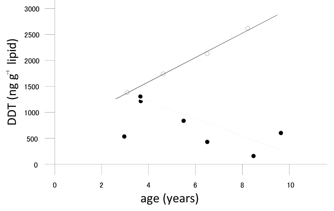
Sex: Chemicals (such as DDT, PCB) accumulated in milk fat may be transferred to juveniles upon lactation. This was found in marine mammals. In this way, females have an additional excretion mechanism. A typical example is shown in Figure 3, taken from a study of Abarnou et al. (1986) on the levels of organochlorinated compounds in the Antarctic dolphin Cephalorhyncus commersonii. In males, concentrations increase with increasing age, but concentrations in mature females decrease with increasing age.
Weight: (body mass) of the organism relative to the surface area across which exchange with the water phase takes place. Smaller organisms have a larger surface-to-volume ratio and the exchange with the surrounding aqueous phase is faster. Therefore, although lipid normalized concentrations will be the same at equilibrium, this equilibrium is reached earlier in smaller than in larger organisms.
Difference in uptake route. The relative importance of uptake through the skin (in fish e.g. the gills) and (oral) uptake through the digestive system. It is generally accepted that for most free-living organism's direct uptake from the water dominates over uptake after digestion in the digestive tract.
Metabolic activity. Even at the same weight or the same age, the balance between uptake and excretion may change due to an increased metabolic activity, e.g. in times of fast growth or high reproductive activity.

alt — Figure 2. The influence of lipid content on the bioconcentration of 1,2,4-trichlorobenzene in different fish species (reproduced using data from Geyer et al., 1985).

Table 1. Mean PCB concentrations in algae (Dunaliella spec.), rotifers (Brachionus plicatilis) and anchovies larvae (Angraulis mordax), expressed on a dry-weight basis and on a lipid basis. From Moriarty (1983).

Organism	Lipid content (%)	PCB-concentration based on dry weight (µg g^-1)	PCB-concentration based on lipid weight (µg g^-1)	BCF based on concentration in the lipid phase
algae	6.4	0.25	3.91	0.48 x 10⁶
rotifer	15.0	0.42	2.80	0.34 x 10⁶
fish (anchovies) larvae	7.5	2.06	27.46	13.70 x 10⁶

alt — Figure 3. Concentrations of DDT in dolphins of different age and the difference between male and female dolphins Redrawn from Abernou et al. (1986) by Wilma IJzerman.

Cited references

Abarnou, A., Robineau, D., Michel, P. (1986). Organochlorine contamination of commersons dolphin from the Kerguelen islands. Oceanologica Acta 9, 19-29.

Armitage, J.M., Arnot, J.A., Wania, F., Mackay, D. (2013). Development and evaluation of a mechanistic bioconcentration model for ionogenic organic chemicals in fish. Environmental Toxicology and Chemistry 32, 115-128.

Geyer, H., Scheunert, I., Korte, F. (1985). Relationship between the lipid-content of fish and their bioconcentration potential of 1,2,4-trichlorobenzene. Chemosphere 14, 545-555.

Mackay, D., Arnot, J.A., Gobas, F., Powell, D.E. (2013). Mathematical relationships between metrics of chemical bioaccumulation in fish. Environmental Toxicology and Chemistry 32, 1459-1466.

Moriarty, F. (1983). Ecotoxicology: The Study of Pollutants in Ecosystems. Publisher: Academic Press, London.

Van der Heijden, S.A., Jonker, M.T.O. (2011). Intra- and interspecies variation in bioconcentration potential of polychlorinated biphenyls: are all lipids equal? Environmental Science and Technology 45, 10408-10414.

Kinetic models

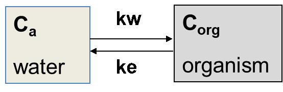
Steady state can be established in a simple laboratory set-up where fish are exposed to a chemical at a constant concentration in the aqueous phase. From the start of the exposure (time 0, or t=0), it will take time for the chemical concentration in the fish to reach steady state and in some cases, this will not be established within the exposure period. In the environment, exposure concentrations may fluctuate and, in such scenarios, constant concentrations in the organism will often not be established. Steady state is reached when the uptake rate (for example from an aqueous phase) equals the elimination rate. Models that include the factor time in describing the uptake of chemicals in organisms are called kinetic models.

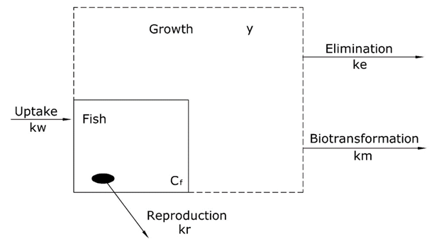
Toxicokinetic models for the uptake of chemicals into fish are based on a number of processes for uptake and elimination. An overview of these processes is presented in Figure 1. In the case of fish, the major process of uptake is by diffusion from the surrounding water compartment via the gill to the blood. Elimination can be via different processes: diffusion via the gill from blood to the surrounding water compartment, via transfer to offspring or eggs by reproduction, by growth (dilution) and by internal degradation of the chemical (biotransformation).

alt — Figure 1. Uptake and elimination processes in fish and the rate constants (k) for each process. Reproduced from Van Leeuwen and Vermeire (2007) by Wilma IJzerman.

Kinetic models to describe uptake of chemicals into organisms are relatively simple with the following assumptions:

First order kinetics:

Rates of exchange are proportional to the concentration. The change in concentration with time (dC / dt ) is related to the concentration and a rate constant (k):

Formule (2)

One compartment:

It is often assumed that an organism consists of only one single compartment and that the chemical is homogeneously distributed within the organism. For "simple" small organisms this assumption is intuitively valid, but for large fish this assumption looks unrealistic. But still, this simple model seems to work well also for fish. To describe the internal distribution of a chemical within fish, more sophisticated kinetic models are needed, similar to the ones applied in mammalian studies. These more complex models are the "physiologically based toxicokinetic" (PBTK) models (Clewell, 1995; Nichols et al., 2004)

Equations for the kinetics of accumulation process

alt

The accumulation process can be described as the sum of rates for uptake and elimination.

Formule (3)

Integration of this differential equation leads to equation 4.

Formule (4)

C_org concentration in organisms (mg/kg)

C_aq concentration in aqueous phase (mg/L)

k_w uptake rate constant (L/kg·day)

k_e elimination rate constant (1/day)

t time (day)

(dimensions used are: amount of chemical: mg; volume of water: L; weight of organism: kg; time: day); see box.

Box: The units of toxicokinetic rate constants

The differential equation underlying toxicokinetic analysis is basically a mass balance equation, specifying conservation of mass. A mass balance implies that the amount of chemical is expressed in absolute units such as mg. If Q is the amount in the animal and F the amount in the environmental compartment the mass balance reads:

Formule

where is the uptake rate constant and k₂ the elimination rate constant, both with dimension time^-1. However, it is often more practical to work with the concentration in the animal (e.g. expressed in mg/kg). This can be achieved by dividing the left and right sides of the equation by w, the body-weight of the animal and defining C_in_t = Q/w. In addition, we define the external concentration as C_env = F/V, where V is the volume (L or kg) of the environmental compartment. This leads to the following formulation of the differential equation:

Formule

Beware that C_env is measured in other units (mg per kg of soil, or mg per litre of water) than C_int (mg per kg of animal tissue). To get rid of the awkward factor V/w it is convenient to define a new rate constant, k₁:

Formule

This is the uptake rate constant usually reported in scientific papers. Note that it has other units than : it is expressed as kg of soil per kg of animal tissue per time unit (kg kg^-1 h^-1), and in the case of water exposure as L kg^-1 h^-1. The dimension of k₂ remains the same whether mass or concentrations are used (time^-1). We also learn from this analysis that when dealing with concentrations, the body-weight of the animal must remain constant.

References

Moriarty, F. (1984) Persistent contaminants, compartmental models and concentration along food-chains. Ecological Bulletins 36: 35-45.

Skip, B., A.J. Bednarska, & R. Laskowski (2014) Toxicokinetics of metals in terrestrial invertebrates: making things straight with the one-compartment principle. PLoS ONE 9(9): e108740.

Equation 4 describes the whole process with the corresponding graphical representation of the uptake graph (Figure 2).

alt — Figure 2. The basic equation for uptake of a chemical from the aqueous phase to a fish: one compartment model with first order kinetics.

The concentration in the organism is the result of the net process of uptake and elimination. At the initial phase of the accumulation process, elimination is negligible and the ratio of the concentration in the organism is given by:

Formule (5)

Formule (6)

Steady state

After longer exposure time, elimination becomes more substantial and the uptake curve starts to level off. At some point, the uptake rate equals the elimination rate and the ratio C_org/C_aq becomes constant. This is the steady state situation. The constant C_org/C_aq at steady state is called the bioconcentration factor BCF. Mathematically, the BCF can also be calculated from k_w/k_e. This follows directly from equation 4: after long exposure time (t), Formule becomes 0 leading to

Formule

Formule (7)

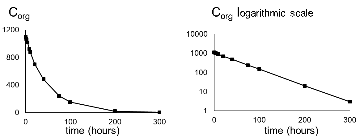
Elimination

Elimination is often measured following an uptake experiment. After the organism has reached a certain concentration, fish are transferred to a clean environment and concentration in the organism will decrease in time. Because this is also a first order kinetic process, the elimination rate will depend on the concentration in the organism (C_org) and the elimination rate constant (k_e) (see equation 8). Concentration will decrease exponentially in time (equation 9) as shown in Figure 3A. Concentrations are often transformed to the natural logarithmic values (ln C_org) because this results in a linear relationship with slope -k_e.(equation 10 and figure 3B).

Formule (8)

Formule (9)

Formule (10)

where C_org(t=0) is the concentration in the organism when the elimination phase starts.

The half-life (T_1/2 or DT₅₀) is the time needed to eliminate half the amount of chemical from the compartment. The relationship between k_e and T_1/2 is: T_1/2 = (In 2) / k_e. The half-life increases when k_e decreases.

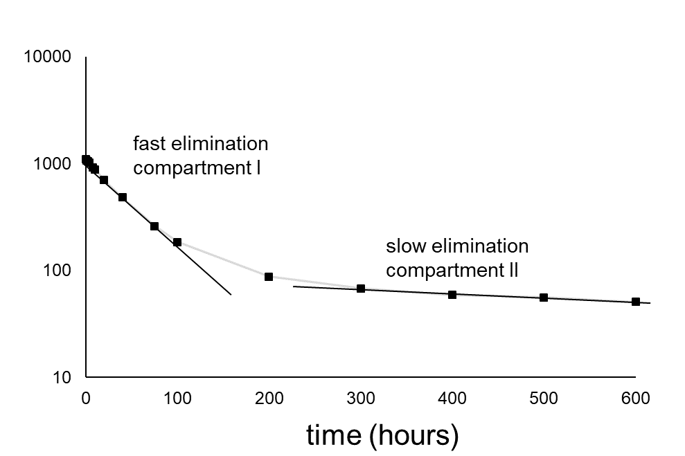
alt — Figure 3. Elimination of a chemical from fish to water: one compartment model. Left: concentrations given on a normal scale. Right: concentration expressed as the natural logarithm to enable linear regression against time to yield the rate constant as the slope.

Multicompartment models

Very often, organisms cannot be considered as one compartment, but as two or even more compartments (Figure 4A). Deviations from the one-compartment system usually are seen when elimination does not follow an exponential pattern as expected: no linear relationship is obtained after logarithmic transformation. Figure 4B shows the typical trend of the elimination in a two-compartment system. The decrease in concentration (on a logarithmic scale) shows two phases: phase I with a relatively fast decrease and phase II with a relatively slow decrease. According to the linear compartment theory, elimination may be described as the sum of two (or more) exponential terms, like:

Formule (11)

where

k_e(I) and k_e(II) represent elimination rate constants for compartment I and II,

F(I) and F(II) are the size of the compartments (as fractions)

Typical examples of two compartment systems are:

Blood (I) and liver (II)
Liver tissue (I) and fat tissue (II)

Elimination from fat tissue is often slower than from, for example, the liver. The liver is a well perfused organ while the exchange between lipid tissue and blood is much less. That explains the faster elimination from the liver.

alt

alt — Figure 4. Elimination of chemical from fish to water (top) in a two-compartment model (bottom).

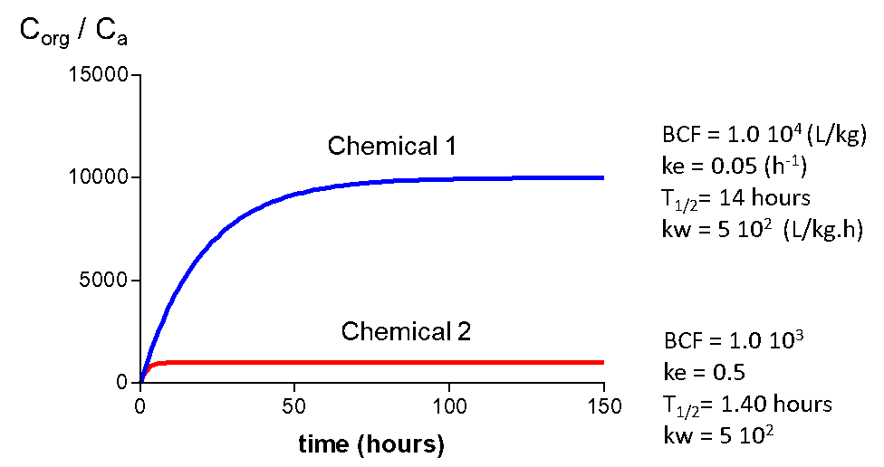
Examples of uptake curves for different chemicals and organisms

Figure 5 gives uptake curves for two different chemicals and the corresponding kinetic parameters. Chemical 2 has a BCF of 1000, chemical 1 a BCF of 10,000. Uptake rates (k_w) are the same, which is often the case for organic chemicals. Half-lives (time to reach 50 % of the steady state level) are 14 and 140 hours. This makes sense because it will take a longer time to reach steady state for a chemical with a higher BCF. Elimination rate constants also differ a factor of 10.

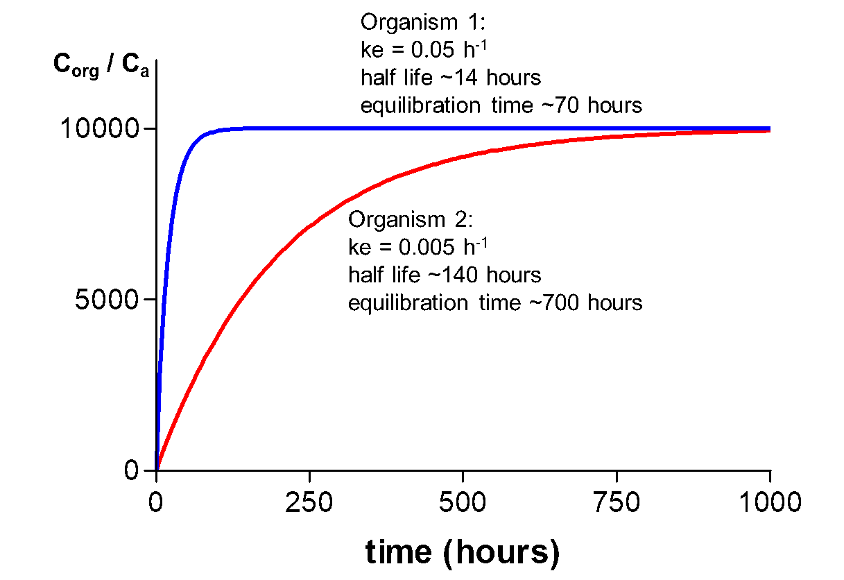
In figure 6, uptake curves are presented for one chemical, but in two organisms of different size/weight. Organism 1 is much smaller than organism 2 and reaches steady state much earlier. T_1/2 values for the chemical in organisms 1 and 2 are 14 and 140 hours, respectively. The small size explains this fast equilibration. Rates of uptake depend on the surface-to-volume ratio (S/V) of an organism, which is much higher for a small organism. Therefore, kinetics in small organisms is faster resulting in shorter equilibration times. The effect of size on kinetics is discussed in more detail in Hendriks et al. (2001) and in the Section on Allometric Relationships.

alt — Figure 5. Uptake curves for two chemicals, having different properties, in the same organism.

alt — Figure 6. Uptake curves for the same chemical in two organisms having different sizes; organism 2 is much bigger than organism 1.

Bioaccumulation involving biotransformation and different routes of uptake

In equation 2, elimination only includes gill elimination. If other processes such as biotransformation and growth are considered, the equation can be extended to include these additional processes (see equation 12).

Formule (12)

For organisms living in soil or sediment, different routes of uptake may be of importance: dermal (across the skin), or oral (by ingestion of food and/or soil or sediment particles). Mathematically, the uptake in an organism in sediment can be described as in equation 13.

Formule (13)

C_org concentration in organisms (mg/kg)

C_aq concentration in aqueous phase (mg/L)

C_s concentration soil or sediment (mg/kg)

k_w uptake rate constant from water (L/kg/day)

k_s uptake rate constant from soil or sediment (kg_soil/kg_organism/day)

k_e elimination rate constant (1/day)

t time (day)

(dimensions used are: amount of chemical: mg; volume of water: L; weight of organism: kg; time: day)

In this equation, k_w and k_s are the uptake rate constants from water and sediment, k_e is the elimination rate constant and C_aq and C_s are the concentrations in water and sediment or soil. For soil organisms, such as earthworms, oral uptake appears to become more important with increasing hydrophobicity of the chemical (Jager et al., 2003). This is because the concentration in soil (C_s) will become higher than the porewater concentration C_a for the more hydrophobic chemicals (see section on Sorption).

References

Clewell, H.J., 3rd (1995). The application of physiologically based pharmacokinetic modeling in human health risk assessment of hazardous substances. Toxicology Letters 79, 207-217.

Hendriks, A.J., van der Linde, A., Cornelissen, G., Sijm, D. (2001). The power of size. 1. Rate constants and equilibrium ratios for accumulation of organic substances related to octanol-water partition ratio and species weight. Environmental Toxicology and Chemistry 20, 1399-1420.

Jager, T., Fleuren, R., Hogendoorn, E.A., De Korte, G. (2003). Elucidating the routes of exposure for organic chemicals in the earthworm, Eisenia andrei (Oligochaeta). Environmental Science and Technology 37, 3399-3404.

Nichols, J.W., Fitzsimmons, P.N., Whiteman, F.W. (2004). A physiologically based toxicokinetic model for dietary uptake of hydrophobic organic compounds by fish - II. Simulation of chronic exposure scenarios. Toxicological Sciences 77, 219-229.

Van Leeuwen, C.J., Vermeire, T.G. (Eds.) (2007). Risk Assessment of Chemicals: An Introduction. Springer, Dordrecht, The Netherlands.

4.1.2. Question 1

What are the assumptions in a one-compartment kinetic model?

4.1.2. Question 2

How can you identify when more compartments are involved in a kinetic model?

4.1.2. Question 3

Give examples of compartments in a multi-compartment system.

4.1.2. Question 4

Why is equilibrium reached faster in a small organism compared to a bigger organism?

4.1.2. Question 5

Which two methods can be applied to estimate the bioconcentration factor of a chemical in an organism?

4.1.3. Tissue accumulation of metals

Author: Nico M. van Straalen

Reviewers: Philip S. Rainbow, Henk Schat

Learning objectives:

You should be able to

indicate four types of inorganic metal binding cellular constituents present in biological tissues and indicate which metals they bind.
describe how phytochelatin and metallothionein are induced by metals.
mention a number of organ-metal combinations that are critical to metal toxicity.

Key words: Metal binding proteins; phytochelatin; metallothionein;

Synopsis

The issue of metal speciation, which is crucially important to understand metal fate in the environment, is equally important for internal distribution in organisms and toxicity inside the cell. Many metals tend to accumulate in specific organs, for example the hepatopancreas of crustaceans, the chloragogen tissue of annelids, and the kidney of mammals. In addition, there is often a specific organ or tissue where dysfunction or toxicity is first observed, e.g., in the human body, the primary effects of chronic exposure to mercury are seen in the brain, for lead in bone marrow and for cadmium in the kidney. This module is aimed at increasing the insight into the different mechanisms by which metals accumulate in biological tissues.

Introduction

Metals will be present in biological tissues in a large variety of chemical forms: free metal ion, various inorganic species with widely varying solubility, such as chlorides or carbonates, plus all kind of metal species bound to low-molecular and high-molecular weight biotic ligands. The free metal ion is considered the most relevant species relating to toxicity.

To explain the affinities of metals with specific targets, a system has been proposed based on the physical properties of the ion; according to this system, metals are divided into "oxygen-seeking metals" (class A, e.g. lithium, beryllium, calcium and lanthanum), and "sulfur-seeking metals" (class B, e.g. silver, mercury and lead) (See section on Metals and metalloids). However, most of the metals of environmental relevance fall in an intermediate class, called "borderline" (chromium, cadmium, copper, zinc, etc.). This classification is to some extent predictive of the binding of metals to specific cellular targets, such as SH-groups in proteins, nitrogen in histidine or carbonates in bone tissue.

Not only do metals differ enormously in their physicochemical properties, also the organisms themselves differ widely in the way they deal with metals. The type of ligand to which a metal is bound, and how this ligand is transported or stored in the body, determines to a great extent where the metal will accumulate and cause toxicity. Sensitive targets or critical biochemical processes differ between species and this may also lead to differential toxicity.

Inorganic metal binding

Many tissues contain "mineral concretions", that is, granules with a specific mineral composition that, due to the nature of the mineral, attract different metals. Especially the gut epithelium of invertebrates, and their digestive glands (hepatopancreas, midgut gland, chloragogen tissue) may be full of such concretions. Four classes of granules are distinguished (Figure 1):

Calcium-pyrophosphate granules with magnesium, manganese, often also zinc, cadmium, lead and iron
Sulfur granules with copper, sometimes also cadmium
Iron granules, containing exclusively iron
Calcium carbonate granules, containing mostly calcium

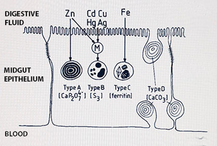
alt — Figure 1. Schematic diagram of the gut epithelium of an invertebrate animal, showing four different types of granules and the metals they usually contain. Redrawn from Hopkin (1989) by Wilma IJzerman.

The type B granules are assumed to be lysosomal vesicles that have absorbed metal-loaded peptides such as metallothionein or phytochelatin, and have developed into inorganic granules by degrading almost all organic material; the high sulfur content derives from the cysteine residues in the peptides.

Tissues or cells that specialize in the synthesis of intracellular granules are also the places where metals tend to accumulate. Well-known are the "S cells" in the hepatopancreas of isopods. These cells (small cells, B-type cells sensu Hopkin 1989) contain very large amounts of copper. Most likely the large stores of copper in woodlice and other crustaceans relate to their use of hemocyanin, a copper-dependent protein, as an oxygen-transporting molecule. Similar tissues with high loadings of mineral concretions have been described for earthworms, snails, collembolans and insects.

Organic metal binding

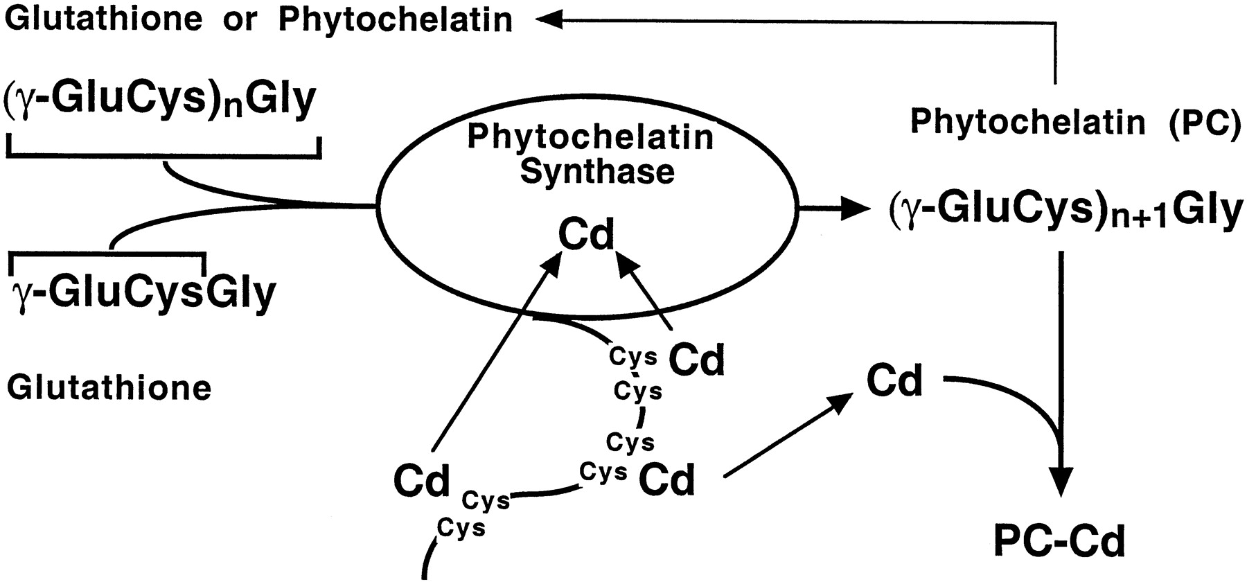
The second class of metal-binding ligands is of organic nature. Many plants but also several animals synthesize a peptide called phytochelatin (PC). This is an oligomer derived from glutathione with the three amino acids, γ-glumatic acid, cysteine and glycine, arranged in the following way: (γ-glu-cys)_n-gly, where n can vary from 2 to 11. The thiol groups of several cysteine residues are involved in metal binding.

The other main organic ligand for metals is metallothionein (MT). This is a low-molecular weight protein with hydrophilic properties and an unusually large number of cysteine residues. Several cysteines (usually nine or ten) can bind a number of metal ions (e.g. four or five) in one cluster. There are two such clusters in the vertebrate metallothionein. Metallothioneins occur throughout the tree of life, from bacteria to mammals, but the amino acid sequence, domain structure and metal affinities vary enormously and it is doubtful whether they represent a single evolutionary-homologous group.

In addition to these two specific classes of organic ligands, MT and PC, metals will also bind aspecifically to all kind of cellular constituents, such as cell wall components, albumen in the blood, etc. Often this represents the largest store of metals; such aspecific binding sites will constantly deliver free metal ions to the cellular pool and so are the most important cause of toxicity. Of course metals are also present in molecules with specific metal-dependent functions, such as iron in hemoglobin, copper in hemocyanin, zinc in carbonic anhydrase, etc.

The distinction between inorganic ligands and organic ones is not as strict as it may seem. After binding to metallothionein or phytochelatin metals may be transferred to a more permanent storage compartment, such as the intracellular granules mentioned above, or they may be excreted.

Regulation of metal binding

Free metal ions are strong inducers of stress response pathways. This can be due to the metal ion itself but more often the stress response is triggered by a metal-induced disturbance of the redox state, i.e. an induction of oxidative stress. The stress response often involves the synthesis of metal-binding ligands such as phytochelatin and metallothionein. Because this removes metal ions from the active pool it is also called metal scavenging.

The binding capacity of phytochelatin is enhanced by activation of the enzyme phytochelatin synthase (PC synthase). According to one model of its action, the C-terminus of the enzyme has a "metal sensor" consisting of a number of cysteines with free SH-groups. Any metal ions reacting with this nucleophile center (and cadmium is a strong reactant) will activate the enzyme which then catalyzes the reaction from (γ-glu-cys)_n-gly to (γ-glu-cys)_n+1-gly, thus increasing the binding capacity of cellular phytochelatin (Figure 2). This reaction of course relies on the presence of sufficient glutathione in the cell. In plants the PC-metal complex is transported into the central vacuole, where it can be stabilized through incorporation of acid-labile sulfur (S²). The PC moiety is degraded, resulting in the formation of inorganic metal-sulfide crystallites. Alternatively, complexes of metals with organic acids may be formed (e.g. citrates or oxalates). The fate of metal-loaded PC in animal cells is not known, but it might be absorbed in the lysosomal system to form B-type granules (see above).

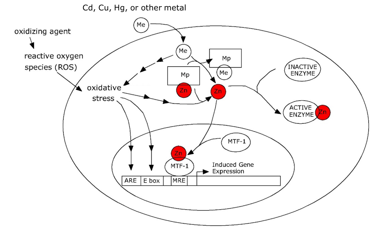
alt — Figure 2. Model for the regulation of phytochelatin synthase, an enzyme catalyzing the extension of phytochelatin and increasing the binding capacity for metals. From Cobbet (2000). Source: http://www.plantphysiol.org/content/123/3/825

The upregulation of metallothionein (MT) occurs in a quite different manner, since it depends on de novo synthesis of the apoprotein. It is a classic example of gene regulation contributing to protection of the cell. In a wide variety of animals, including vertebrates and invertebrates, metallothionein genes (Mt) are activated by a transcription factor called metal-responsive transcription factor 1 (MTF-1). MTF -1 binds to so-called metal-responsive elements (MREs) in the promoter of Mt. MREs are short motives with a characteristic base-pair sequence that form the core of a transcription factor binding site in the DNA. Under normal physiological conditions MTF-1 is inactive and unable to induce Mt. However, it may be activated by Zn²⁺ ions, which are released, from unspecified ligands, by metals such as cadmium that can replace zinc (Figure 3).

alt — Figure 3. Model for metallothionein induction by cadmium. Cadmium ions (Me) displace zinc ions from ligands (MP). Free zinc ions (Zn) then activate Metal Transcription Factor 1 (MTF-1) in the nucleus to bind to transcription factor binding sites containing Metal-Responsive Elements (MRE). This induces expression of Mt and other genes. These genes may also be induced by oxidative stress, acting upon antioxidant-responsive elements (ARE) and Enhancer Box (E box). Oxidative stress may come from external oxidizing agents or from the metal itself. Finally, zinc ions may also directly activate antioxidant enzymes. Adapted from Haq et al. (2003) by Wilma IJzerman.

It must be emphasized that the model discussed above is inspired by work on vertebrates. Arthropods (Drosophila, Orchesella, Daphnia) could have a similar mechanism since they also have an MTF-1 homolog that activates Mt, however, the situation for other invertebrates such as annelids and gastropods is unclear; their Mt genes seem to lack MREs, despite being inducible by cadmium. In addition, the variability of metallothioneins in invertebrates is extremely large and not all metal-binding proteins may be orthologs of the vertebrate metallothionein. In snails, a cadmium-binding, cadmium-induced MT functions alongside a copper-binding MT while the two MTs have different tissue distributions and are also regulated quite differently.

While both phytochelatin and metallothionein will sequester essential as well as non-essential metals (e.g. Cd) and so contribute to detoxification, the widespread presence of these systems throughout the tree of life suggests that they did not evolve primarily to deal with anthropogenic metal pollution. The very strong inducibility of these systems by non-essential elements like cadmium may be considered a side-effect of a different primary function, for example regulation of the cellular redox state or binding of essential metals.

Target organs

Any tissue-specific accumulation of metals can be explained by turnover of metal-binding ligands. For example, accumulation of cadmium in mammalian kidney is due to the fact that metallothionein loaded with cadmium cannot be excreted. High concentrations of metals in the hind segments of earthworms are due to the presence of "residual bodies" which are fully packed with intracellular granules. Accumulation of cadmium in the human prostrate is due to the high concentration of zinc citrate in this organ, which serves to protect contractile proteins in sperm tails from oxidation; cadmium assumedly enters the prostrate through zinc transporters.

It is often stated that essential metals are subject to regulatory mechanisms, which would imply that their body burden, over a large range of external exposures, is constant. However, not all "essential" metals are regulated to the extent that the whole-body concentration is kept constant. Many invertebrates have body compartments associated with the gut (midgut gland, hepatopancreas, Malpighian tubules) in which metals, often in the form of mineral concretions, are inactivated and stored permanently or exchanged very slowly with the active pool. Since these compartments are outside the reach of regulatory mechanisms but usually not separated in whole-body metal analysis, the body burden as a whole is not constant. Some invertebrates even carry a "backpack" of metals accumulating over life. This holds, e.g., for zinc in barnacles, copper in isopods and zinc in earthworms.

Accumulation of metals in target organs may lead to toxicity when the critical binding or excretion capacity is exhausted and metal ions start binding aspecifically to cellular constituents. The organ in which this happens is often called the target organ. The total metal concentration at which toxicity starts to become apparent is called the critical body concentration (CBC) or critical tissue concentration. For example, the critical concentration for cadmium in kidney, above which renal damage is observed to occur, is estimated to be 50 μg/g. A list of critical organs for metals in the human body is given in Table 1.

The concept of CBC assumes that the complete metal load in an organ is in equilibrium with the active fraction causing toxicity and that there is no permanent storage pool. In the case of storage detoxification the body burden at which toxicity appears will depend on the accumulation history.

Table 1. Critical organs for chronic toxicity of metals in the human body

Metal or metalloid	Critical organ	Symptoms
Al	Brain	Alzheimer's disease
As	Lung, liver, heart gut	Multisystem energy disturbance
Cd	Kidney, liver	Kidney damage
Cr	Skin, lung, gut	Respiratory system damage
Cu	Liver	Liver damage
Hg	Brain, liver	Mental illness
Ni	Skin, kidney	Allergic reaction, kidney damage
Pb	Bone marrow, blood, brain	Anemia, mental retardation

References

Cobbett, C., Goldsbrough, P. (2002). Phytochelatins and metallothioneins: roles in heavy metal detoxification and homeostasis. Annual Review of Plant Biology 53, 159-182.

Dallinger, R., Berger, B., Hunziker, P., Kägi, J.H.R. (1997). Metallothionein in snail Cd and Cu metabolism. Nature 388, 237-238.

Dallinger, R., Höckner, M. (2013). Evolutionary concepts in ecotoxicology: tracing the genetic background of differential cadmium sensitivities in invertebrate lineages. Ecotoxicology 22, 767-778.

Haq, F., Mahoney, M., Koropatnick, J. (2003) Signaling events for metallothionein induction. Mutation Research 533, 211-226.

Hopkin, S.P. (1989) Ecophysiology of Metals in Terrestrial Invertebrates. London, Elsevier Applied Science.

Nieboer, E., Richardson, D.H.S. (1980) The replacement of the nondescript term "heavy metals" by a biologically and chemically significant classification of metal ions. Environmental Pollution Series B 1, 3-26.

Rainbow, P.S. (2002) Trace metal concentrations in aquatic invertebrates: why and so what? Environmental Pollution 120, 497-507.

4.1.3. Question 1

Mention the four main inorganic cellular constituents that bind metals, their main elemental composition and indicate what metals are usually bound in each structure.

4.1.3. Question 2

How can the intracellular levels of metal-scavenging molecules such as metallothionein (MT) and phytochelatin (PC) be adjusted to counteract the possible adverse effects of free metal ions? Describe the molecular mechanism for metallothionein and phytochelatin separately.

4.1.3. Question 3

Mention three organs of the human body susceptible to metal intoxication and to which metals they are particularly sensitive.

4.1.4. Xenobiotic defence and metabolism

Author: Nico M. van Straalen

Reviewers: Timo Hamers, Cristina Fossi

Learning objectives:

You should be able to:

recapitulate the phase I, II and III mechanisms for xenobiotic metabolism, and the most important molecular systems involved.
describe the fate and the chemical changes of an organic compound that is metabolized by the human body, from absorption to excretion.
explain the principle of metabolic activation and why some compounds can become very reactive upon xenobiotic metabolism.
develop a hypothesis on the ecological effects of xenobiotic compounds that require metabolic activation.

Keywords: biotransformation; phase 1; phase II; phase III; excretion; metabolic activation; cytochrome P450

Synopsis

All organisms are equipped with metabolic defence mechanisms to deal with foreign compounds. The reactions involved, jointly called biotransformation, can be divided into three phases, and usually aim to increase water solubility and excretion. The first step (phase I) is catalyzed by cytochrome P450, which is followed by a variety of conjugation reactions (phase II) and excretion (phase III). The enzymes and transporters involved are often highly inducible, i.e. the amount of protein is greatly enhanced by the xenobiotic compounds themselves. The induction involves binding of the compound to cytoplasmic receptor proteins, such as the arylhydrocarbon receptor (AhR), or the constitutive androstane receptor (CAR). In some cases the intermediate metabolites, produced in phase I are extremely reactive and a main cause of toxicity, a well-known example being the metabolic activation of polycyclic aromatic hydrocarbons such as benzo(a)pyrene, which readily forms DNA adducts and causes cancer. In addition, some compounds greatly induce metabolizing enzymes but are hardly degraded by them and cause chronic cellular stress. The various biotransformation reactions are a crucial aspect of both toxicokinetics and toxicodynamics of xenobiotics.

Introduction

The term "xenobiotic" ("foreign to biology") is generally used to indicate a chemical compound that does not normally have a metabolic function. We will use the term extensively in this module, despite the fact that it is somewhat problematic (e.g., can a compound be considered "foreign" if it circulates in the body, is metabolized or degraded in the body?, and: what is "foreign" for one species is not necessarily "foreign" for another species).

The body has an extensive defence system to deal with xenobiotic compounds, loosely designated as biotransformation. The ultimate result of this system is excretion the compound in some form or another. However, many xenobiotics are quite lipophilic, tend to accumulate and are not easily excreted due to low water solubility. Molecular modifications are usually required before such compounds can be removed from the body, as the main circulatory and excretory systems (blood, urine) are water-based. By introducing hydrophilic groups in the molecule (-OH, =O, -COOH) and by conjugating it to an endogenous compound with good water-solubility, excretion is usually accomplished. However, as we will see below, intermediate metabolites may have enhanced reactivity and it often happens that a compound becomes more toxic while being metabolized. In the case of pesticides, deliberate use is made of such responses, to increase the toxicity of an insecticide once it is in the target organism.

The study of xenobiotic metabolism is a classical subject not only in toxicology but also in pharmacology. The mode of action of a drug often depends critically on the rate and mode of metabolism. Also, many drugs show toxic side-effects as a consequence of metabolism. Finally, xenobiotic metabolism is also studied extensively in entomology, as both toxicity and resistance of pesticides are often mediated by metabolism.

The most problematic xenobiotics are those with a high octanol-water partition coefficient (K_ow) that are strongly lipophilic and very hydrophobic. They tend to accumulate, in proportion to their Log K_ow, in tissues with a high lipid content such as the subcutis of vertebrates, and may cause tissue damage due to disturbance of membrane functions. This mode of action is called "minimum toxicity". Well-known are low-molecular weight aliphatic petroleum compounds and chlorinated alkanes such as chloroform. These compounds cause their primary damage to cell membranes; especially neurons are sensitive to this effect, hence minimum toxicity is also called narcotic toxicity. Lipophilic chemicals with high Log K_ow do not reach concentrations high enough to cause minimum toxicity because they induce biotransformation at lower concentrations. The toxicity is then usually due to a reactive metabolite.

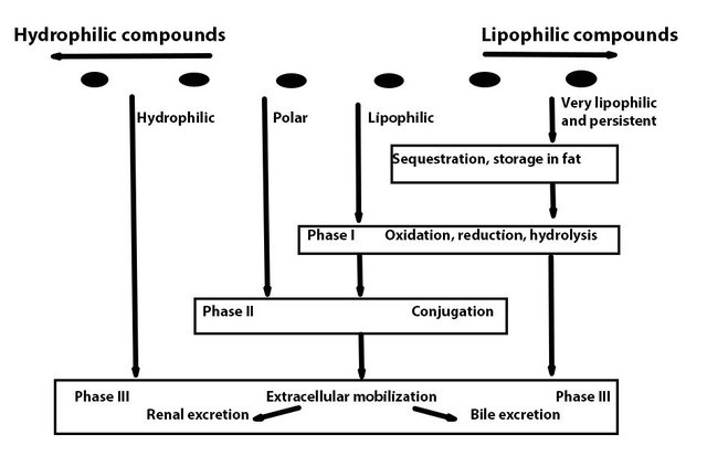
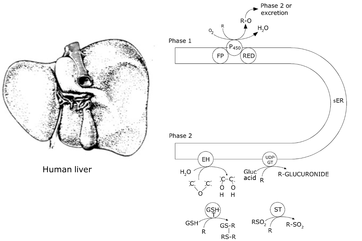
Xenobiotic metabolism involves three subsequent phases (Figure 1):

Activation (usually oxidation) of the compound by an enzyme known as cytochrome P450, which acts in cooperation with NADPH cytochrome P450 reductase and other factors.
Conjugation of the activated product of phase I to an endogenous compound. A host of different enzymes is available for this task, depending on the compound, the tissue and the species. There are also (slightly polar) compounds that enter phase II directly, without being activated in phase I.
Excretion of the compound into circulation, urine, or other media, usually by means of membrane-spanning transporters belonging to the class of ATP-binding cassette (ABC) transporters, including the infamous multidrug resistance proteins. Hydrophilic compounds may pass on directly to phase III, without being activated or conjugated.

alt — Figure 1. The various phases of xenobiotic metabolism. Redrawn by Wilma Ijzerman.

Phase I reactions

Cytochrome P450 is a membrane-bound enzyme, associated with the smooth endoplasmic reticulum. It carries a porphyrin ring containing an Fe atom, which is the active center of the molecule. The designation P450 is derived from the fact that it shows an absorption maximum at 450 nm when inhibited by carbon monoxide, a now outdated method to demonstrate its presence. Other (outdated) namings are MFO (mixed function oxygenase) and drug metabolizing enzyme complex. Cytochrome P450 is encoded by a gene called CYP, of which there are many paralogs in the genome, all slightly differing from each other in terms of inducibility and substrate specificity. Three classes of CYP genes are involved with biotransformation, designated CYP1, CYP2 and CYP3 in vertebrates. Each class has several isoforms; the human genome has 57 different CYP genes in total. The CYP complement of invertebrates and plants often involves even more genes; many evolutionary lineages have their own set, arising from extensive gene duplications within that lineage. In humans, the genetic complement of a person's CYP genes is highly relevant as to its drug metabolizing profile (see the section on Genetic variation in toxicant metabolism).

Cytochrome P450 operates in conjunction with an enzyme called NADPH cytochrome P450 reductase, which consists of two flavoproteins, one containing Flavin adenine dinucleotide (FAD), the other flavin mononucleotide (FMN). The reduced Fe²⁺ atom in cytochrome P450 binds molecular oxygen, and is oxidized to Fe³⁺ while splitting O₂; one O atom is introduced in the substrate, the other reacts with hydrogen to form water. Then the enzyme is reduced by accepting an electron from cytochrome P450 reductase. The overall reaction can be written as:

RH + O₂ + NADPH + H⁺ → ROH + H₂O + NADP⁺

where R is an arbitrary substrate.

Cytochrome P450 is expressed to a great extent in hepatocytes (liver cells), the liver being the main organ for xenobiotic metabolism in vertebrates (Figure 2), but it is also present in epithelia of the lung and the intestine. In insects the activity is particularly high in the Malpighian tubules in addition to the gut and the fat body. In mollusks and crustaceans the main metabolic organ is the hepatopancreas.

Phase II reactions

After activation by cytochrome P450 the oxidized substrate is ready to be conjugated to an endogenous compound, e.g. a sulphate, glucose, glucuronic acid or glutathione group. These reactions are conducted by a variety of different enzymes, of which some reside in the sER like P450, while others are located in the cytoplasm of the cell (Figure 2). Most of them transfer a hydrophilic group, available from intermediate metabolism, to the substrate, hence the enzymes are called transferases. Usually the compound becomes more polar in phase II, however, not all phase II reactions increase water solubility; for example, methylation (by methyl transferase) decreases reactivity but increases apolarity. Other phase II reactions are conjugation with glutathione, conducted by glutathione-S-transferase (GST) and with glucuronic acid, conducted by UDP-glucuronyl transferase. In invertebrates other conjugations may dominate, e.g. in arthropods and plants, conjugation with malonyl glucose is a common reaction, which is not seen in vertebrates.

Conjugation with glutathione in the human body is often followed by splitting off glutamic acid and glycine, leaving only the cysteine residue on the substrate. Cysteine is subsequently acetylated, thus forming a so-called mercapturic acid. This is the most common type of metabolite for many xenobiotics excreted in urine by humans.

Like cytochrome P450, the phase II enzymes consist in various isoforms, encoded by different paralogs in the genome. Especially the GST family is quite extensive and polymorphisms in these genes contribute significantly to the personal metabolic profile (see the section on Genetic variation in toxicant metabolism).

alt — Figure 2. Schematic view of xenobiotic metabolism (phase I and phase II) in human liver. P450 = cytochrome P450, FP = flavoprotein, RED = cytochrome P450 reductase, EH = epoxide hydrolase, UDP-GT = uridyldiphospho-glucuronyl transferase, GSH-T = glutathione-S-transferase, ST = sulphotransferase. Reproduced from Vermeulen & Van den Broek (1984) by Wilma Ijzerman.

Phase III reactions

In the human body, there are two main pathways for excretion, one from the liver into the bile (and further into the gut and the faeces), the other through the kidney and urine. These two pathways are used by different classes of xenobiotics: very hydrophobic compounds such as high-molecular weight polycyclic aromatic hydrocarbons are still not readily soluble in water even after metabolism but can be emulsified by bile salt and excreted in this way. It sometimes happens that such compounds, once arriving in the gut, are assimilated again, transported to the liver by the portal vein and metabolized again. This is called "entero-hepatic circulation". Lower molecular weight compounds and hydrophilic compounds are excreted through urine. Volatile compounds can leave the body through the skin and exhaled air.

Excretion of activated and conjugated compounds from tissues out of the cell usually requires active transport, which is mediated by ABC (ATP binding cassette) transporters, a very large and diverse family of membrane proteins which have in common a binding cassette for ATP. Different subgroups of ATP transporters transport different types of chemicals, e.g. positively charged hydrophobic molecules, neutral molecules and water-soluble anionic compounds. One well-known group consists of multidrug resistance proteins or P-glycoproteins. These transporters export drugs aiming to attack tumor cells. Because their activity is highly inducible, these proteins can enhance excretion enormously, making the cell effectively resistant and thus case major problems for cancer treatment.

Induction

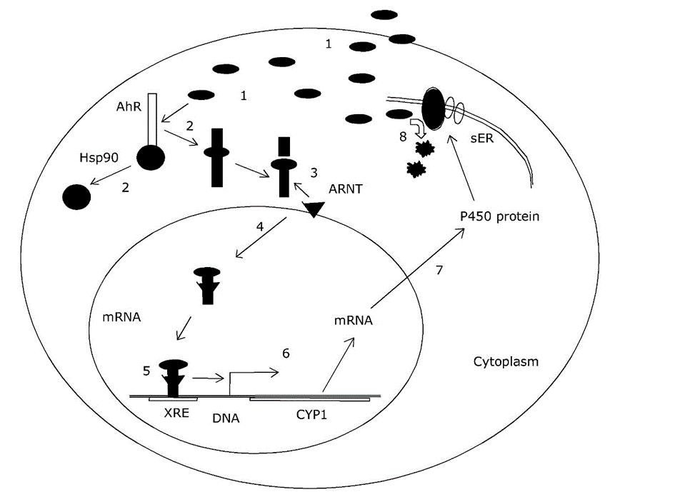
All enzymes of xenobiotic metabolism are highly inducible: their activity is normally on a low level but is greatly enhanced in the presence of xenobiotics. This is achieved through a classic case of transcriptional regulation upon CYP and other genes, leading to de novo synthesis of protein. In addition, extensive proliferation of the endoplasmic reticulum may occur, and in extreme cases even swelling of the liver (hepatomegaly).

The best investigated pathway for transcriptional activation of CYP genes is due to the arylhydrocarbon receptor (AhR). Under normal conditions, this peptide is stabilized in the cytoplasm by heat-shock proteins, however, when a xenobiotic compound binds to AhR, it is activated and can join with another protein called Ah receptor nuclear translocator (ARNT) to translocate to the nucleus and bind to DNA elements present in the promotor of CYP and other genes. It thus acts as a transcriptional activator or transcription factor on these genes (Figure 3). The DNA motifs to which AhR binds are called xenobiotic responsive elements (XRE) or dioxin-responsive elements (DRE). The compounds acting in this manner are called 3-MC-type inducers, after the (highly carcinogenic) model compound 3-methylcholanthrene. The inducing capacity of a compound is related to its binding affinity to the AhR, which in itself is determined by the spatial structure of the molecule. The lock-and key fitting between AhR and xenobiotics explains why induction of biotransformation by xenobiotics shows a very strong stereospecificity. For example, among the chlorinated biphenyls and chlorinated dibenzodioxins, some compounds are extremely strong inducers of CYP1 genes, while others, even with the same number of chlorine atoms, are no inducers at all. The precise position of the chlorine atoms determines the molecular "fit" in the Ah receptor (see Section on Receptor interaction).

In addition to 3MC-type of induction there are other modes in which biotransformation enzymes are induced, but these are less well-known. A common class is PB-type induction (named after another model compound, phenobarbital). PB-type induction is not AhR-dependent, but acts through activation of another nuclear receptor, called constitutive androstane receptor (CAR). This receptor activates CYP2 genes and some CYP3 genes.

The high inducibility of biotransformation can be exploited in a reverse manner: if biotransformation is seen to be highly upregulated in a species living in the environment, this indicates that that species is being exposed to xenobiotic compounds. Assays addressing cytochrome P450 activity can therefore be exploited in bioindication and biomonitoring systems. The EROD (ethoxyresorufin-O-deethylase) assay is often used for this purpose, although it is not 100% specific to the isoform of P450. Another approach is to address CYP expression directly, e.g. through reverse transcription-quantitative PCR, a method to quantify the amount of CYP mRNA.

alt — Figure 3. Scheme illustrating how AhR-reactive compounds induce biotransformation activity. 1 xenobiotic compounds enter the cell through diffusion, 2 compound binds to AhR, releasing it from Hsp90, 3 AhR complex is activated by ARNT, 4 translocation to nucleus, 5 binding to XRE, 6 enhanced transcription, 7 translocation of mRNA to cytoplasm and translation, 8 incorporation of P450 enzyme in sER and biotransformation of compounds. AhR = arylhydrocarbon receptor, Hsp90 = heat shock protein 90, ARNT = aryl hydrocarbon nuclear translocator, XRE = xenobiotic responsive element, CYP1 = gene encoding cytochrome P450 1, sER = smooth endoplasmic reticulum. Drawn by Wilma Ijzerman.

Secondary effects of biotransformation

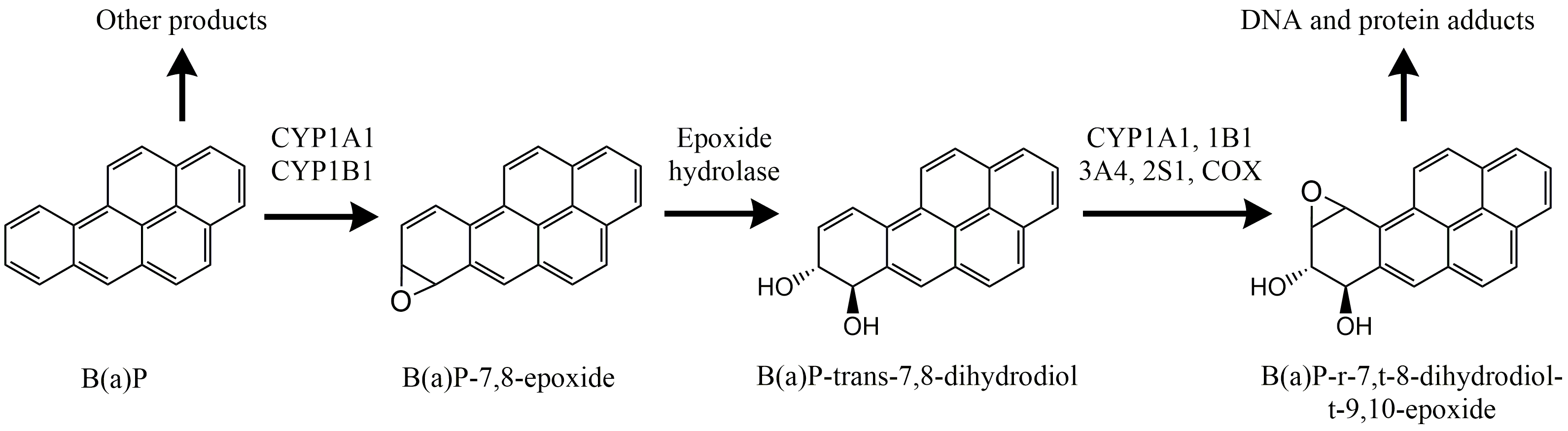
Although the main aim of xenobiotic metabolism is to detoxify and excrete foreign compounds, some pathways of biotransformation actually enhance toxicity. This is mostly due to the first step, activation by cytochrome P450. The activation may lead to intermediate metabolites which are highly reactive and the actual cause of toxicity. The best investigated examples are due to bioactivation of polycyclic aromatic hydrocarbons (PAHs), a group of chemicals present in diesel, soot, cigarette smoke and charred food products. Many of these compounds, e.g. benzo(a)pyrene, benz(a)anthracene and 3-methylcholanthrene, are not reactive or toxic as such but are activated by cytochrome P450 to extremely reactive molecules. Benzo(a)pyrene, for instance, is activated to a diol-epoxide, which readily binds to DNA, especially to the free amino-group of guanine (Figure 4). The complex is called a DNA adduct, the double helix is locally disrupted and this results in a mutation. If this happens in an oncogene, a tumor may develop (see the Section on Carcinogenesis and genotoxicity).

Not all PAHs are carcinogenic. Their activity critically depends on the spatial structure of the molecule, which again determines its "fit" in the Ah receptor. PAHs with a "notch" (often called bay-region) in the molecule tend to be stronger carcinogens than compounds with a symmetric (round or linear) molecular structure.

alt — Figure 4. Metabolism of benzo(a)pyrene (B[a]P) to a mutagenic and carcinogenic metabolite, BaP-diol epoxide. Cytochrome P450 activity (CYP1A1 and CYP1B1) introduces an epoxide on the 7,8 position of the molecule, which is then hydrolyzed by epoxide hydrolase to a dihydrodiol (two OH groups next to each other, which can be in trans position, pointing in different directions relative to the plane of the molecule, or in cis, pointing in the same direction). The trans metabolite is preferably formed. Subsequently another epoxide is introduced on the 9,10 position. The diolepoxide is highly reactive, and may bind proteins and to guanine in DNA, causing a DNA adduct. Modified from Bui et al. (2009) by Steven Droge.

Another mechanism for biotransformation-induced toxicity is due to some very recalcitrant organochlorine compounds such as polychlorinated dibenzodioxins (PCDDs, or dioxins for short) and polychlorinated biphenyls (PCBs). Some of these compounds are very potent inducers of biotransformation, but they are hardly degraded themselves. The consequence is that the highly upregulated cytochrome P450 activity continues to generate a large amount of reactive oxygen (ROS), causing oxidative stress and damage to cellular constituents. It is assumed that the chronic toxicity of 2,3,7,8-tetrachlorodibenzo(para)dioxin (TCDD), one of the most toxic compounds emitted by human activity, is due to its high capacity to induce prolonged oxidative stress. On the molecular level, there is a close link between oxidative stress and biotransformation activity. Many toxicants that primarily induce oxidative stress (e.g. cadmium) also upregulate CYP enzymes. Two defence mechanisms, oxidative stress defence and biotransformation are part of the same integrated stress defence system of the cell.

References

Bui, P.H., Hsu, E.L., Hankinson, O. (2009), Fatty acid hydroperoxides support cytochrome P450 2S1-mediated bioactivation of benzo[a]pyrene-7-8-dihydrodiol. Molecular Pharmacology 76, 1044-1052.

Stroomberg, G.J., Zappey, H., Steen, R.J.C.A., Van Gestel, C.A.M., Ariese, F., Velthorst, N.H., Van Straalen, N.M. (2004). PAH biotransformation in terrestrial invertebrates - a new phase II metabolite in isopods and springtails. Comparative Biochemistry and Physiology Part C 138, 129-137.

Timbrell, J.A. (1982). Principles of Biochemical Toxicology. Taylor & Francis Ltd, London.

Van Straalen, N.M., Roelofs, D. (2012). An Introduction to Ecological Genomics, 2^nd Ed. Oxford University Press, Oxford.

Vermeulen, N.P.E., Van den Broek, J.M. (1984). Opname en verwerking van chemicaliën in de mens. Chemisch Magazine. Maart: 167-171.

4.1.4. Question 1

Describe the main processes involved with each of the three general phases of xenobiotic metabolism, as well as the molecular systems involved.

4.1.4. Question 2

The upregulation of cytochrome P450 activity is a classical example of regulation through enhanced de novo synthesis of enzyme. The mechanism is known in quite some detail and involves a variety of components. Describe the involvement of the following components

Aryl hydrocarbon receptor
Heat shock protein 70
Arylhydrocarbon receptor nuclear translocator
Xenobiotic-response elements
CYP1A1 gene
CYP1A1 mRNA
CYP 1A1 protein
CYP 1A1 enzymatic activity

4.1.4. Question 3

In the past, activity of cytochrome P450 was often assessed using a synthetic fluorescent substrate, resorufin; activity was measured as ethoxyresorufin-O-deethylase (EROD). Discuss the advantages and disadvantages of the use of such an assay in environmental risk assessment.

4.1.5. Allometric relationships

Author: A. Jan Hendriks

Reviewers: Nico van den Brink, Nico van Straalen

Learning objectives:

You should be able to

explain why allometrics is important in risk assessment across chemicals and species
summarize how biological characteristics such as consumption, lifespan and abundance scale size
describe how toxicological quantities such as uptake rates and lethal concentrations scale to size

Keywords: body size, biological properties, scaling, cross-species extrapolation, size-related uptake kinetics

Introduction

Globally more than 100,000,000 chemicals have been registered. In the European Union more than 100,000 compounds are awaiting risk assessment to protect ecosystem and human health, while 1,500,000 contaminated sites potentially require clean-up. Likewise, 8,000,000 species, of which 10,000 are endangered, need protection worldwide, with one lost per hour (Hendriks, 2013). Because of financial, practical and ethical (animal welfare) constraints, empirical studies alone cannot cover so many substances and species, let alone their combinations. Consequently, the traditional approach of ecotoxicological testing is gradually supplemented or replaced by modelling approaches. Environmental chemists and toxicologists for long have developed relationships allowing extrapolation across chemicals. Nowadays, so-called Quantitative Structure Activity Relationships (QSARs) provide accumulation and toxicity estimates for compounds based on their physical-chemical properties. For instance bioaccumulation factors and median lethal concentrations have been related to molecular size and octanol-water partitioning, characteristic properties of a chemical that are usually available from its industrial production process.

In analogy with the QSAR approach in environmental chemistry, the question may be asked whether it is possible to predict toxicological, physiological and ecological characteristics of species from biological traits, especially traits that are easily measured, such as body size. This approach has gone under the name "Quantitative Species Sensitivity Relationships" (QSSR) (Notenboom, 1995).

Among the various traits available, body-size is of particular interest. It is easily measured and a large part of the variability between organisms can be explained from body size, with r² > 0.5. Not surprisingly, body size also plays an important role in toxicology and pharmacology. For instance, toxic endpoints, such as LC₅₀s, are often expressed per kg body weight. Recommended daily intake values assume a "standard" body weight, often 60 kg. Yet, adult humans can differ in body weight by a factor of 3 and the difference between mouse and human is even larger. Here it will be explored how body-size relationships, which have been studied in comparative biology for a long time, affect the extrapolation in toxicology and can be used to extrapolate between species.

Fundamentals of scaling in biology

Do you expect a 10⁴ kg elephant to eat 10⁴ times more than a 1 kg rabbit per day? Or less, or more? On being asked, most people intuitively come up with the right answer. Indeed, daily consumption by the proboscid is less than 10⁴ times that of the rodent. Consequently, the amount of food or water used per kilogram of body weight of the elephant is less than that of the rabbit. Yet, how much less exactly? And why should sustaining 1 kg of rabbit tissue require more energy than 1 kg of elephant flesh in the first place?

A century of research (Peters, 1983) has demonstrated that many biological characteristics Y scale to size X according to a power function:

Y = a X^b

where the independent variable X represents body mass, and the dependent variable Y can virtually be any characteristic of interest ranging, e.g., from gill area of fish to density of insects in a community.

Plotted in a graph, the equation produces a curved line, increasing super-linearly if b > 1 and sub-linearly if b < 1. If b=1, Y and X are directly proportional and the relationship is called isometric. As curved lines are difficult to interpret, the equation is often simplified by taking the logarithm of the left and right parts. The formula then becomes:

log Y = log a + b log X

When log Y is plotted against log X, a straight line results with slope b and intercept log a. If data are plotted in this way, the slope parameter b may be estimated by simple linear regression.

Across wide size ranges, slope b often turns out to be a multitude of ¼ or, occasionally, ⅓. Rates [kg∙d^-1] of consumption, growth, reproduction, survival and what not, increase with mass to the power ¾ , while rate constants, sometimes called specific rates [kg∙kg^-1∙d^-1], decrease with mass to the power -¼. So, while the elephant is 10⁴ kg heavier than the 1 kg rabbit, it eats only (10⁴)^¾ = 10³ times more each day. Vice versa, 1 kg of proboscid apparently requires a consumption of (10⁴)^-¼ kg∙kg^-1∙d^-1, i.e., 10 times less. Variables with a time dimension [d] like lifespan or predator-prey oscillation periods scale inversely to rate constants and thus change with body mass to the power ¼. So, an elephant becomes (10⁴)^¼ = 10 times older than a rabbit. Abundance, i.e., the number of individuals per surface area [m^-2] decreases with body mass to the power -¾. Areas, such as gill surface or home range, scale inversely to abundance, typically as body mass to the power ¾.

Now, why would sustaining 1 kg of elephant require 10 times less food than 1 kg of rabbit? Biologists, pharmacologists and toxicologists first attributed this difference to area-volume relationships. If objects of the same shape but different size are compared, the volume increases with length to the power 3 and the surface increases with length to the power 2. For a sphere with radius r, for example, area A and volume V increase as A ~ r² and V ~ r³, so area scales to volume as A ~ r² ~ (V^⅓)² ~ V^⅔. So, larger animals have relatively smaller surfaces, as long as the shape of the organism remains the same. Since many biological processes, such as oxygen and food uptake or heat loss deal with surfaces, metabolism was, for long, thought to slow down like geometric structures, i.e., with multitudes of ⅓. Yet, empirical regressions, e.g. the "mouse-elephant curve" developed by Max Kleiber in the early 1930s show a universal slope of ¼ (Peters, 1983. This became known as the "Kleiber's law". While the data leave little doubt that this is the case, it is not at all clear why it should be ¼ and not ⅓. Several explanations for the ¼ slope have been proposed but the debate on the exact value as well as the underlying mechanism continues.

Application of scaling in toxicology

Since chemical substances are carried by flows of air and water, and inside the organism by sap and blood, toxicokinetics and toxicodynamics are also expected to scale to size. Indeed, data confirm that uptake and elimination rate constants decrease with size, with an exponent of about -¼ (Figure 1). Slopes vary around this value, the more so for regressions that cover small size ranges and physiologically different organisms. The intercept is determined by resistances in unstirred water layers and membranes through which the substances pass, as well as by delays in the flows by which they are carried. The resistances mainly depend on the affinity and molecular size of the chemicals, reflected by, e.g., the octanol-water partition coefficient K_ow for organic chemicals or atomic mass for metals. The upper boundary of the intercept is set by the delays imposed by consumption and, subsequently, egestion and excretion. The lower end is determined by growth dilution. Both uptake and elimination scale to mass with the same exponent so that their ratio, reflecting the bioconcentration or biomagnification factor in equilibrium, is independent of body-size.

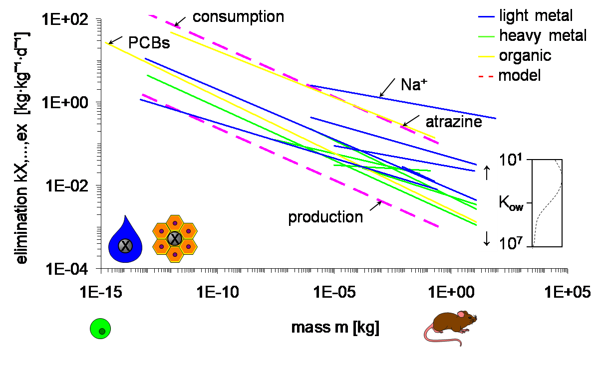
alt — Figure 1. Regressions of elimination rate constants [kg∙kg^-1∙d^-1 = d^-1] as a function of organism mass m [kg], ranging from algae to mammals, and organic chemicals' octanol-water partition ratio K_ow and metal mass within the limits set by consumption and production (redrawn by author, based on Hendriks et al. 2001).

Scaling of rate constants for uptake and elimination, such as in Figure 1, implies that small organisms reach a given internal concentration faster than large ones. Vice versa, lethal concentrations in water or food needed to reach the same internal level after equal (short-term) exposure duration are lower in smaller compared to larger organisms. Thus, the apparent "sensitivity" of daphnids can, at least partially, be attributed to their small body-size. This emphasizes the need to understand simple scaling relationships before developing to more elaborate explanations.

Using Figure 1, one can, within strict conditions not elaborated here, theoretically relate median lethal concentrations LC₅₀ [μg L^-1] to the K_ow of the chemical and the size of the organism, with r² > 0.8 (Hendriks, 1995; Table 1). Complicated responses like susceptibility to toxicants can be predicted only from K_ow and body size, which illustrates the generality and power of allometric scaling. Of course, the regressions describe the general trends and in individual cases the deviations can be large. Still, considering the challenges of risk assessment as outlined above, and in the absence of specific data, the predictions in Table 1 can be considered as a reasonable first approximation.

Table 1. Lethal concentrations and doses as a function of test animal body-mass

Species	Endpoint	Unit	b (95% CI)	r²	n_c	n_s	Source
Guppy	LC₅₀	mg∙L^-1	0.66 (0.51-0.80)	0.98	6	1	1
Mammals	LD₁₀≈MTD	mg∙animal^-1	0.73	0.69‑0.77	27	5	2
Birds	Oral LD₅₀	mg∙animal^-1	1.19 (0.67-0.82)	0.76	194	3…37	3
Mammals	Oral LD₅₀	mg∙animal^-1	0.94 (1.18-1.20)	0.89	167	3…16	4
Mammals	Oral LD₅₀	mg∙animal^-1	1.01 (1.00-1.01)		>5000	2…8	5

MTD = maximum threshold dose, repeated dosing. LD₅₀ single dose, b = slope of regression line, n_c = number of chemicals, n_s = number of species. Sources: 1 Anderson & Weber (1975), 2 Travis & White (1987), 4 Sample & Arenal (1999), 5 Burzala-Kowalczyk & Jongbloed (2011).

Allometry is also important when dealing with other levels of biological organisation. Leaf or gill area, the number of eggs in ovaries, the number of cell types and many other cellular and organ characteristics scale to body-size as well. Likewise, intrinsic rates of increase (r) of populations and the production-biomass ratios (P/B) of communities can also be obtained from the (average) species mass. Even the area needed by animals in laboratory assays scales to size, i.e., by m^¾, approximately the same slope noted for home ranges of individuals in the field.

Future perspectives

Since almost any physiological and ecological process in toxicokinetics and toxicodynamics depends on species size, allometric models are gaining interest. Such an approach allows one to quantitatively attribute outliers (like apparently "sensitive" daphnids) to simple biological traits, rather than detailed chemical-toxicological mechanisms.

Scaling has been used in risk assessment at the molecular level for a long time. The molecular size of a compound is often a descriptor in QSARs for accumulation and toxicity. If not immediately evident as molecular mass, volume or area often pops up as an indicator of steric properties. Scaling does not only apply to bioaccumulation and toxicity from molecular to community levels, size dependence is also observed in other sections of the environmental cause-effect chain. Emissions of substances, e.g., scale non-linearly to the size of engines and cities. Concentrations of chemicals in rivers depend on water discharge, which in itself is an allometric function of catchment size. Hence, understanding the principles of cross-disciplinary scaling is likely to pay off in protecting many species against many chemicals.

References

Anderson, P.D., Weber, L.J. (1975). Toxic response as a quantitative function of body size. Toxicology and Applied Pharmacology 33, 471-483.

Burzala-Kowalczyk, L., Jongbloed, G. (2011). Allometric scaling: Analysis of LD50 data. Risk Analysis 31, 523-532.

Hendriks, A.J. (1995). Modelling response of species to microcontaminants: Comparative ecotoxicology by (sub)lethal body burdens as a function of species size and octanol-water partitioning of chemicals. Ecotoxicology and Environmental Safety 32, 103-130.

Hendriks, A.J. (2013). How to deal with 100,000+ substances, sites, and species: Overarching principles in environmental risk assessment. Environmental Science and Technology 47, 3546−3547.

Hendriks, A.J., Van der Linde, A., Cornelissen, G., Sijm, D.T.H.M. (2001). The power of size: 1. Rate constants and equilibrium ratios for accumulation of organic substances. Environmental Toxicology and Chemistry 20, 1399-1420.

Notenboom, J., Vaal, M.A., Hoekstra, J.A. (1995). Using comparative ecotoxicology to develop quantitative species sensitivity relationships (QSSR). Environmental Science and Pollution Research 2, 242-243.

Peters, R.H. (1983). The Ecological Implications of Body Size. Cambridge University Press, Cambridge.

Sample, B.E., Arenal, C.A. (1999) Allometric models for interspecies extrapolation of wildlife toxicity data. Bulletin of Environmental Contamination and Toxicology 62, 653-66.

Travis, C.C., White, R.K. (1988) Interspecific scaling of toxicity data. Risk Analysis 8, 119-125.

4.1.5. Question 1

Think of a biological trait that you are interested in. How do you think it will scale to organism size?

4.1.5. Question 2

What is the elimination rate constant of a chemical with a K_ow of 10⁴ from an insect with a mass of 10^-5 kg?

4.1.5. Question 3

Why is size-scaling more prominent in toxicokinetics than in toxicodynamics?

4.1.6. Food chain transfer

Auteur: Nico van den Brink

Reviewers: Kees van Gestel. Jan Hendriks

Learning objectives:

You should be able to:

Mention the chemical properties determining the potential of chemicals to accumulate in food chains
Explain the role of biological and ecological factors in the food-chain accumulation of chemicals

Keywords: biomagnification, food-chain transfer,

Accumulation of chemicals across different trophic levels.

Chemicals may be transferred from one organism to another. Grazers will ingest chemicals that are in the vegetation they eat. Similarly, predators are exposed to chemicals in their prey items. This so-called food web accumulation is governed by properties of the chemical, but also by some traits of the receiving organism (e.g. grazer or predator).

Chemical properties driving food web accumulation

Some chemicals are known to accumulate in food webs, reaching the highest concentrations in top-predators. Examples of such chemicals are organochlorine pesticides like DDT and brominated flame retardants (e.g. PBDEs; see section on POPs). Such accumulating chemicals have a few properties in common: they need to be persistent and they need to have affinity for the organismal body. Organic chemicals with a relatively high log Kow, indicating a high affinity for lipids, will enter organisms quite effectively (see section on Bioconcentration and kinetics modelling). Once in the body, these chemicals will be distributed to lipid rich tissues, and excretion is rather limited. In case of persistent chemicals that are not metabolised, concentrations will increase over time when uptake is higher than excretion. Furthermore, such chemicals are likely to be passed on to organisms at the next trophic level in case of prey-predator interactions. Some of these chemicals may be metabolised by the organism, most often into more water soluble metabolites (see section on Xenobiotic metabolism & defence). These metabolites are more easily excreted, and in this way concentrations of metabolizable chemicals do not increase so much over time, and will therefore also transfer less to higher trophic levels. The effects of metabolism on the internal concentrations of organisms is clearly illustrated by a study on the uptake of organic chemicals by different aquatic species (Kwok et al., 2013). In that study the uptake of persistent chemicals (organochlorine pesticides; OCPs) was compared with the uptake of chemicals that may be metabolised (polycyclic aromatic hydrocarbons; PAHs). The authors compared shrimps with fish, the former having a limited capacity to metabolise PAHs while fish can. Figure 1 shows the Biota-to-Sediment Accumulation Factors (BSAFs; see section on Bioaccumulation), which is the ratio between the concentration in the organism and in the sediment. It is shown that OCPs accumulate to a high extent in both species, reflecting persistent, non-metabolizable chemicals. For PAHs the results are different per species, fish are able to metabolise and as a result the concentrations of PAHs in the fish are low, while in shrimp, with a limited metabolic capacity, the accumulation of PAHs is comparable to the OCPs. These results show that not only the properties of the chemicals are of importance, but also some traits of the organisms involved, in this case the metabolic capacity.

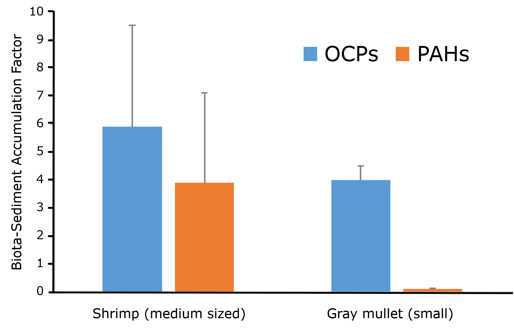
alt — Figure 1. Biota-sediment accumulation factors organochlorine pesticides (OCPs) and polycyclic aromatic hydrocarbons (PAHs) in fish and shrimp. Redrawn from Kwok et al. (2013).

Effects of species traits and food web structure on food web accumulation

Food-web accumulation of chemicals is driven by food uptake. At lower trophic levels, most organisms will acquire relatively low concentrations from the ambient environment. First consumers, foraging on these organisms will accumulate the chemicals of all of them, and in case of persistent chemicals that enter the body easily, concentrations in the consumers will be higher than in their diet. Similarly, concentrations will increase when the chemicals are transferred to the next trophic level. This process is called biomagnification, indicating increasing concentrations of persistent and accumulative chemicals in food webs. The most iconic example of this is on the increasing concentrations of DDTs in fish eating American Osprey (Figure 2), a casus which has led to the ban of a lot of organochlorine chemicals.

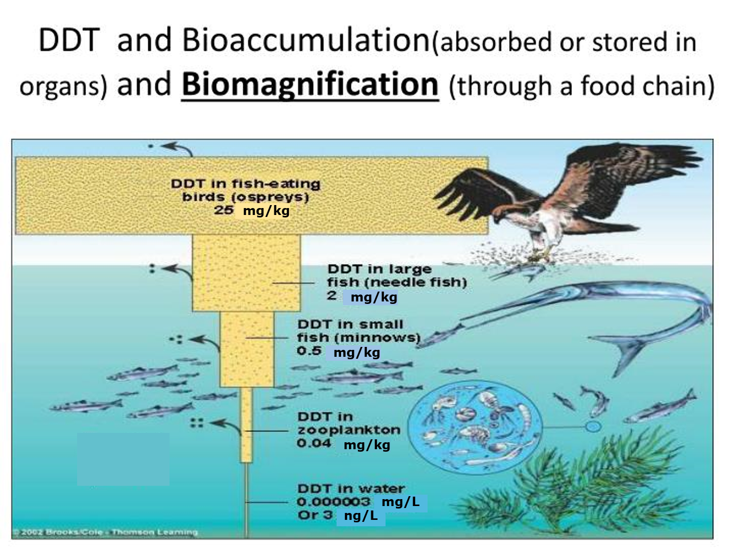
alt — Figure 2. Example of biomagnification of DDT in an aquatic food web of ospreys. Slightly modified from: http://naturalresources.anthro-semin...magnification/.

Since biomagnification along trophic levels is food driven, it is of importance to include diet composition into the studies. This can be explained by an example on small mammals in the Netherlands. Two similar small mammal species, the bank vole (Myodes glareolus) and the common vole (Microtus arvalis) co-occur in larger part of the Netherlands. Although the species look very similar, they are different in their diet and habitat use. The bank vole is a omnivorous species, inhabiting different types of habitat while the common vole is strictly vegetarian living in pastures. In a study on the species-specific uptake of cadmium, diet items of both species were analysed, indicating nearly 3 orders of magnitudes differences in cadmium concentrations between earthworms and berries from vegetation (Fig 3A, van den Brink et al., 2010). Stable isotopic ratios of carbon and nitrogen were used to assess the general diets of the organisms. The common vole ate mostly stinging nettle and grass, including seeds, while the bank vole showed to forage on grass herbs and earthworms. This difference in diet was reflected in increased concentrations of cadmium in the bank vole in comparison to the common vole (both inhabiting the same area). The concentrations of one bank vole appeared to be extremely low (red diamond in Figure 3b), and initially this was considered to be an artefact. However, detailed analysis of the stable isotopic ratios in this individual revealed that it had foraged on stinging nettle and grass, hence a diet more reflecting the common vole. This emphasises once more that organisms accumulate through their diet (you accumulate what you eat!)

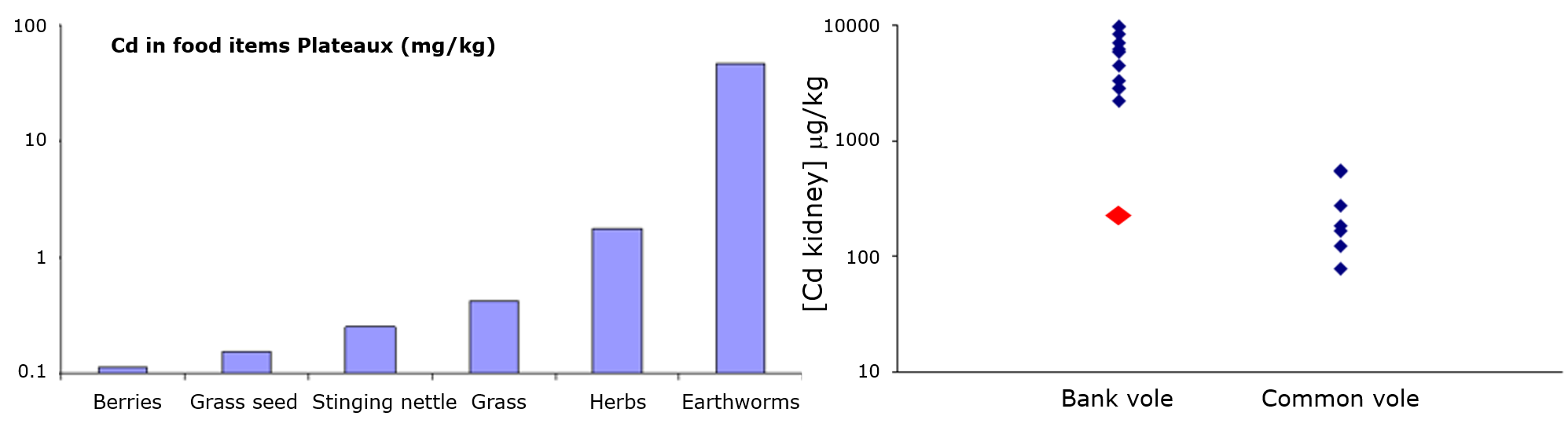
alt — Figure 3. Left: Concentrations of cadmium in diet items of small mammals collected in the Plateaux area near Eindhoven, the Netherlands; Right: Cadmium concentrations in kidneys of bank voles and common voles collected in the Plateaux area. See text for further explanation. Redrawn from van den Brink et al. (2010).

Case studies

Orcas or Killer whales (Orcinus orca) are large marine predatory mammals, which roam all around the oceans, from the Arctic to the deep south region of the Antarctic. Although they appear ubiquitous around the world, generally different pods of Orcas occur in different regions of the marine ecosystem. Often, each pod has developed specialised foraging behaviours targeted at specific prey species. Although Orcas are generally apex top-predators at the top of the (local) food web, the different foraging strategies would suggest that exposure to accumulating chemicals may differ considerably between pods. This was indeed shown to be the case in a very elaborate study on different pods of Orcas of the West-coast of Canada by Ross et al. (2000). In the Vancouver region there is a resident pod while the region is also often visited by two transient groups of Orcas. PCB concentrations were high in all animals, but the transient animals contained significantly higher levels. The transient whales mainly fed on marine mammals, while the resident animals mainly fed on fish, and this difference in diet was thought to be the cause of the differences in PCB levels between the groups. In that study, it was also shown that PCB levels increased with age, due to the persistence of the PCBs, while female orcas contained significant lower concentrations of PCBs. The latter is caused by the lactation of the female Orcas during which they feed their calves with lipid rich milk, containing relatively high levels of (lipophilic) PCBs. By this process, females offload large parts of their PCB body burden, however by transferring these PCBs to their developing calves (see also Figure 3 in the section on Bioaccumulation). A recent study showed that although PCBs have been banned for decades now, they still pose threats to populations of Orcas (Deforges et al., 2018). In that study, regional differences in PCB burdens were confirmed, likely due to differences in diet preferences although not specifically mentioned. It was shown that PCB levels in most of the Orca populations were still above toxic threshold levels and concerns were raised regarding the viability of these populations. This study confirms that 1) Orcas are exposed to different levels of PCBs according to their diet, which influences the biomagnification of the PCBs, 2) Orca populations are very inefficient in clearing PCBs from the individual due to little metabolism but also from the population due to the efficient maternal transfer from mother to calve, and 3) persistent, accumulating chemicals may pose threats to organisms even decades after their use. Understanding the mechanisms and processes underlying the biomagnification of persistent and toxic compounds is essential for a in depth risk assessment.

References

Desforges, J.-P., Hall, A., McConnell, B., Rosing-Asvid, A., Barber, J.L., Brownlow, A., De Guise, S., Eulaers, I., Jepson, P.D., Letcher, R.J., Levin, M., Ross, P.S., Samarra, F., Víkingson, G., Sonne, C., Dietz, R. (2018). Predicting global killer whale population collapse from PCB pollution. Science 361, 1373-1376.

Ford, J.K.B., Ellis, G.A., Matkin, D.R., Balcomb, K.C., Briggs, D., Morton, A.B. (2005). Killer whale attacks on minke whales: Prey capture and antipredator tactics. Marine Mammal Science 21, 603-618.

Guinet, C. (1992). Predation behaviour of killer whales (Orcinus orca) around Grozet Islands. Canadian Journal of Zoology 70, 1656-1667.

Kwok, C.K., Liang, Y., Leung, S.Y., Wang, H., Dong, Y.H., Young, L., Giesy, J.P., Wong, M.H. (2013). Biota-sediment accumulation factor (BSAF), bioaccumulation factor (BAF), and contaminant levels in prey fish to indicate the extent of PAHs and OCPs contamination in eggs of waterbirds. Environmental Science and Pollution Research 20, 8425-8434.

Ross, P.S., Ellis, G.M., Ikonomou, M.G., Barrett-Lennard, L.G., Addison, R.F. (2000). High PCB concentrations in free-ranging Pacific killer whales, Orcinus orca: Effects of age, sex and dietary preference. Marine Pollution Bulletin 40, 504-515.

Samarra, F.I.P., Bassoi, M., Beesau, J., Eliasdottir, M.O., Gunnarsson, K., Mrusczok, M.T., Rasmussen, M., Rempel, J.N., Thorvaldsson, B., Vikingsson, G.A. (2018). Prey of killer whales (Orcinus orca) in Iceland. Plos One 13, 20.

van den Brink, N., Lammertsma, D., Dimmers, W., Boerwinkel, M.-C., van der Hout, A. (2010). Effects of soil properties on food web accumulation of heavy metals to the wood mouse (Apodemus sylvaticus). Environmental Pollution 158, 245-251.

4.1.6. Question 1

In a lake, the ecosystem consists of algae, daphnids feeding on the algae and fish feeding on the daphnids. Chemical A has a low log K_ow, but is persistent. Chemical B has high log K_ow, but can be metabolised by daphnids and fish, and Chemical C has high log K_ow and is also persistent. Where may you find the highest concentrations of Chemical A, B and C?

4.1.6. Question 2

Name the two traits of species determining the potential for chemicals to reach high concentrations in it.

4.1.6. Question 3

This is a more general question, trying to put the information in the text of this section on bioaccumulation across different trophic levels in a broader perspective:

What property does a chemical need, besides high potential for bioaccumulation and persistence, to have a high likelihood to pose serious environmental risks to organisms?

4.1.7. Critical Body Concentration

Author: Martina G. Vijver

Reviewers: Kees van Gestel and Frank Gobas

Learning objectives:

You should be able to

describe the Critical Body Concentration (CBC) concept for assessing the toxicity of chemicals.

graphically explain the CBC concept and make a distinction between slow and fast kinetics.
mention cases in which the CBC approach fails.

Keywords:

Time dependent effects, internal body concentrations, one compartment model

Introduction

One of the quests in ecotoxicology is how to link toxicity to exposure and to understand why some organisms experience toxic effects while others do not at the same level of exposure. A generally accepted approach for assessing possible adverse effects on biota, no matter what kind of species, is the Critical Body Concentration (CBC) concept (McCarty 1991). According to this concept, toxicity is determined by the amount of chemical taken up, so by the internal concentration, which has a relationship with the duration of the exposure as well as the exposure concentration.

Figure 1 shows the relationship between the development with time of the internal concentrations of a chemical in an organism and the time when mortality occurs at different exposure concentrations under constant exposure. Independent of exposure time or exposure concentration, mortality occurs at a more or less fixed internal concentration. The CBC is defined as the highest internal concentration of a substance in an organism that does cause a defined effect, e.g. 50% mortality or 50% reduction in the number of offspring produced. By comparing internal concentrations measured in exposed organisms to CBC values derived in the laboratory, a measure of risk is obtained. The CBC applies to lethality as well as to sub-lethal effects like reproduction or growth inhibition.

Relating toxicity to toxicokinetics

From Figure 1A, it may also become clear that chemicals that have fast uptake kinetics will reach the CBC faster than chemicals that have slow kinetics (see Section on Bioaccumulation kinetics). As a consequence, also the time to reach a constant LC₅₀ (indicated as the ultimate LC₅₀: LC₅₀¥; Figure 1B) depends on kinetics. Hence, both toxic effects and chemical concentration are controlled by the same kinetics.The CBC can be derived from the LC₅₀-time relationship and be linked to the LC₅₀¥ using uptake and elimination rate constants (k₁ and k₂). It should be noted that the k₂ in this case does not reflect the rate of chemical excretion but rather the rate of elimination of toxic effects caused by the chemical (so, note the difference here with Section on Bioaccumulation kinetics).

alt

alt — Figure 1: A. The relationship between uptake kinetics of a chemical in an organism and its toxicity according to the Critical Body Concentration (CBC) concept under constant exposure. The red line depicts the highest internal concentration of the chemical in the organism killing the organism (CBC); exceedance of that line results in mortality. B. The relationship between LC₅₀ and time. LC₅₀ will reach a constant value with time, indicated as the ultimate LC₅₀ (LC₅₀¥). The CBC can be calculated from the LC₅₀¥ using uptake and elimination rate constants (k₁ and k₂) derived by first order kinetics as shown here. Note: the CBC approach is not limited to first order kinetics. And the same curves may be seen when focusing on sublethal effects, LC₅₀ then reads EC₅₀. Drawn by Wilma Ijzerman.

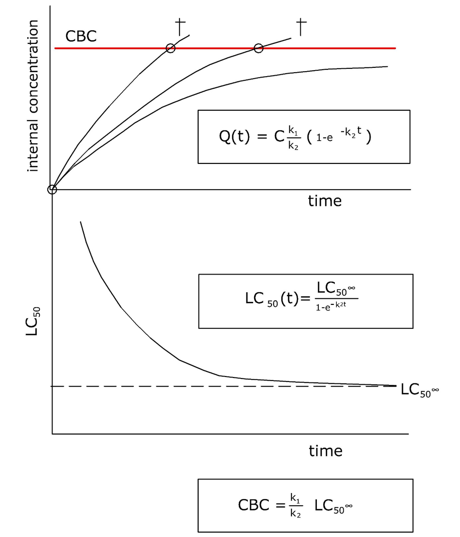
The time needed to reach steady state depends on the body size of the organisms, with larger organisms taking longer time to attain steady state compared to smaller organisms (McCarty 1991). The time needed to reach steady state depends also on the exposure surface area of the exposed organisms (Pawlisz and Peters 1993) as well as their metabolic activity. Organisms not capable of excreting or metabolizing a chemical will continue accumulating with time, and the LC₅₀¥ will be zero. This is e.g. the case for cadmium in isopods (Crommentuijn et al. 1994), but kinetics are so slow that cadmium in these animals never reaches lethal concentrations in relatively clean environments as their life span is too short.

The CBC integrates environmentally available fractions with bioavailable concentrations and toxicity at specific receptors (McCarty and MacKay 1993). See also Section on Bioavailability. In this way, the actual exposure concentration in the environment does not need to be known for performing a risk assessment. The internal concentration of the chemical in the organism is the only concentration required for a risk assessment. Therefore many difficulties are overcome regarding bioavailability issues, e.g. it removes some of the disadvantages of the exposure concentration expressed per unit of soil, as well as of dealing with exposures that vary over time or space.

Proof of the CBC concept

A convincing body of evidence was collected to support the CBC approach. For organic compounds with a narcotic mode of action, effects could be assessed over a wide range of organisms, test compounds and exposure media. For narcotic compounds with octanol-water partition coefficients (K_ow) varying from 10 to 1,000,000 (see for details Section on Relevant chemical properties), the concentration of chemical required for lethality through narcosis is approximately 1-10 mmol/kg: Figure 2 (McCarty and MacKay 1993).

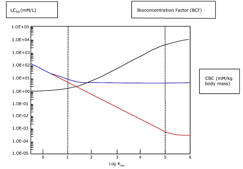
alt — Figure 2: Theoretical plot supporting the Critical Body Concentration (CBC) concept for non-polar organic chemicals acting by narcosis. The bioconcentration factor (BCF in L/kg body mass; black line) of these chemicals increases with increasing log K_ow while their acute toxicity also increases (LC₅₀ in test solution in mM decreases; red line). The product of LC₅₀ and BCF is the critical body concentrations (in mM/kg body mass; blue line). Adapted from McCarty and Mackay (1993) by Wilma Ijzerman.

To reduce the variation in bioconcentration factor (BCF) values for the accumulation of chemicals in organisms from water, normalization by lipid content has been suggested allowing to determine the chemical activity within an organism's body (US EPA 2003). For that reason, lipid extraction protocols are intensively described within the updated OECD Guideline for the testing of chemicals No. 305 for fish bioaccumulation tests, along with a sampling schedule of lipid measurement in fish. Correction of the BCF for differences in lipid content is also described in the same OECD guideline No. 305. If chemical and lipid analyses have been conducted on the same fish, this requires correction for the corresponding lipid content of each individual measured concentration in the fish. This should be done prior to using the data to calculate the kinetic BCF. If lipid content is not measure on all sampled fish, a mean lipid content of approx. 5% must be used to normalize the BCF. It should be noted that this correction holds only for chemicals accumulating in lipids and not for chemicals that do primarily bind to proteins (e.g. perfluorinated substances).

When does the CBC concept not apply?

The CBC concept also has some limitations. Crommentuijn et al. (1994) found that the toxicity of metals to soil invertebrates could not be explained using critical body concentrations. The way different organisms deal with accumulated metals has a large impact on the magnitude of body concentrations reached and the accompanying metal sensitivity (Rainbow 2002). Moreover, adaptation or development of metal tolerance limits the application of CBCs for metals. When the internal metal concentration does not show a monotonic relationship with the exposure concentration, it is not possible to derive CBCs. This means that whenever organisms are capable of trapping a portion of the metal in forms that are not biologically reactive, a direct relationship between body metal concentrations and toxicity may be absent or less evident (Luoma and Rainbow 2005, Vijver et al. 2004). Consequently, for metals a wide range of body concentrations with different biological significance exists. It therefore remains an open question whether the approach is applicable to modes of toxic action other than narcosis. Another important point is the question to what extent the CBC approach is applicable to assessing the effect of chemical mixtures, especially in cases the chemicals have a different mode of action.

References

Crommentuijn, T., Doodeman, C.J.A.M., Doornekamp, A., Van der Pol, J.J.C., Bedaux, J.J.M., Van Gestel, C.A.M. (1994). Lethal body concentrations and accumulation patterns determine time-dependent toxicity of cadmium in soil arthropods. Environmental Toxicology and Chemistry 13, 1781-1789.

Luoma, S.N., Rainbow, P.S. (2005). Why is metal bioaccumulation so variable? Biodynamics as a unifying concept. Environmental Science and Technology 39, 1921-1931

McCarty, L.S. (1991). Toxicant body residues: implications for aquatic bioassays with some organic chemicals. In: Mayes, M.A., Barron, M.G. (Eds.), Aquatic Toxicology and Risk Assessment: Fourteenth Volume. ASTM STP 1124. Philadelphia: American Society for Testing and Materials. pp. 183-192. DOI: 10.1520/STP23572S

McCarty, L.S., Mackay, D. (1993). Enhancing ecotoxicological modeling and assessment. Environmental Science and Technology 27, 1719-1727

Pawlisz, A.V., Peters, R.H. (1993). A test of the equipotency of internal burdens of nine narcotic chemicals using Daphnia magna. Environmental Science and Technology 27, 2801-2806

Rainbow P.S. (2002). Trace metal concentrations in aquatic invertebrates: why and so what? Environmental Pollution 120, 497-507.

U.S. EPA. (2003). In: Methodology for Deriving Ambient Water Quality Criteria for the Protection of Human Health: Technical Support Document. Volume 2. United States Environmental Protection Agency, Washington, D.C: Development of National Bioaccumulation Factors.

Vijver M.G., Van Gestel, C.A.M., Lanno, R.P., Van Straalen, N.M., Peijnenburg, W.J.G.M. (2004) Internal metal sequestration and its ecotoxicological relevance: a review. Environmental Science and Technology 18, 4705-4712.

4.1.7. Question 1

Explain why the CBC approach integrates chemical and biological availability.

4.1.7. Question 2

How are time dynamics involved in the CBC approach?

4.1.7. Question 3

Under what conditions the CBC approach cannot be applied?

4.1. Toxicokinetics

4.1.1. Bioaccumulation

Introduction: terminology for bioaccumulation

Caq concentration in water (aqueous phase)

Corg concentration in organism

Cf concentration in food

Cs concentration in sediment or soil

Effect of biological properties on accumulation

Factors related to the organism are:

DBW

DSL-W

DML-W

fSL

fML

fNLOM

fW

Cited references

Suggested reading

4.1.2. Toxicokinetics

Kinetic models

First order kinetics:

One compartment:

Equations for the kinetics of accumulation process

References

Steady state

Elimination

Multicompartment models

Examples of uptake curves for different chemicals and organisms

Bioaccumulation involving biotransformation and different routes of uptake

References

4.1.3. Tissue accumulation of metals

Synopsis

Introduction

Inorganic metal binding

Organic metal binding

Regulation of metal binding

Target organs

References

4.1.4. Xenobiotic defence and metabolism

Synopsis

Introduction

Phase I reactions

Phase II reactions

Phase III reactions

Induction

Secondary effects of biotransformation

References

4.1.5. Allometric relationships

Introduction

Fundamentals of scaling in biology

Application of scaling in toxicology

MTD = maximum threshold dose, repeated dosing. LD50 single dose, b = slope of regression line, nc = number of chemicals, ns = number of species. Sources: 1 Anderson & Weber (1975), 2 Travis & White (1987), 4 Sample & Arenal (1999), 5 Burzala-Kowalczyk & Jongbloed (2011).

Future perspectives

References

4.1.6. Food chain transfer

Accumulation of chemicals across different trophic levels.

Chemical properties driving food web accumulation

Effects of species traits and food web structure on food web accumulation

Case studies

References

4.1.7. Critical Body Concentration

Introduction

Relating toxicity to toxicokinetics

Proof of the CBC concept

When does the CBC concept not apply?

References

C_aq concentration in water (aqueous phase)

C_org concentration in organism

C_f concentration in food

C_s concentration in sediment or soil

D_BW

D_SL-W

D_ML-W

f_SL

f_ML

f_NLOM

f_W

MTD = maximum threshold dose, repeated dosing. LD₅₀ single dose, b = slope of regression line, n_c = number of chemicals, n_s = number of species. Sources: 1 Anderson & Weber (1975), 2 Travis & White (1987), 4 Sample & Arenal (1999), 5 Burzala-Kowalczyk & Jongbloed (2011).