
3.1: Environmental compartments
- Page ID
- 294544

3.1.1. Introduction
In order to understand and predict the effects of chemicals in the environment we need to understand the behaviour of chemicals in specific environments and in the environment as a whole. In order to deal with the diversity of natural systems, we consider them to consist of compartments. These are defined as parts of the physical environment that are defined by a spatial boundary that distinguishes them from the rest of the world, for example the atmosphere, soil, surface water and even biota. These examples suggest that three phases: gas, liquid, and solid, are important but compartments may consist of different phases. For example, the atmosphere consists of suspended liquids (e.g., fog) and solids (e.g., dust) as well as gases. Similarly, lakes contain suspended solids and soils contain gaseous and water-filled pore space. In detailed environmental models, each of these phases may also be considered to be a compartment.
The behaviour and fate of chemicals in the environment is determined by the properties of environmental compartments and the physicochemical characteristics of the chemicals. Together these properties determine how chemicals undergo chemical and biological reactions, such as hydrolysis, photolysis and biodegradation, and phase transfer processes such as air-water exchange and sorption.
In this chapter, we first introduce the most important compartments and their most important properties and processes that determine the behaviour of chemical contaminants: the atmosphere, the hydrosphere, sediment, soil, groundwater and biota. The emissions of chemicals into the environment from either point sources or diffuse sources is discussed and the important pathways and processes determining the fate of chemicals. The partitioning approach to phase-transfer processes is presented with sorption as a specific example. The impact of physicochemical properties on partitioning is also discussed.
Other important environmental processes are discussed in sections on metal speciation, processes affecting the bioavailability of metals and organic contaminants and the transformation and degradation of organic chemicals. These sections also include information on the basic methods to measure these processes.
Finally, approaches that are used to model and predict the environmental fate of chemicals, and thus the exposure of organisms to these chemicals are described in section 3.8.
3.1.2. Atmosphere
Authors: Astrid Manders-Groot
Reviewer: Kees van Gestel, John Parsons, Charles Chemel
Leaning objectives:
You should be able to:
- describe the structure of the atmosphere and mention its main components
- describe the processes that determine residence time and transport distances of chemicals in air
Keywords: atmosphere, transport distance, residence time
Composition and vertical structure of atmosphere
The atmosphere of the Earth consists of several layers that have limited interaction. The troposphere is the lowermost part of the atmosphere and contains the oxygen that we breathe and most of the water vapor. It contains on average 78% N2, 20% O2 and up to 4% water vapor. Greenhouse gases like CO2 and CH4 are present at 0.0038 % and 0.0002%, respectively. Air pollutants like ozone and NO2 have concentrations that are even a factor 1,000-10,000 lower, but are already harmful for the health of humans, animals and vegetation at these concentrations.
The troposphere is 6-8 km high near the poles, about 10 km at mid-latitudes and about 15 km at the equator. It has its own circulation and determines what we experience as weather, with temperature, wind, clouds and precipitation. The lowest part of the troposphere is the boundary layer, the part that is closest to the Earth. Its height is determined by the heating of the atmosphere by the Earth surface and the wind conditions and has a daily cycle, determined by the incoming sunlight. It is not a completely separate layer, but the exchange of air pollutants like O3, NOx, SO2, and xenobiotic chemicals between the boundary layer and the above layers is generally inefficient. Therefore it is also termed the mixing layer.
Above the troposphere there is the stratosphere, a layer that is less strongly influenced by the daily solar cycle. It is very dry and has its owns circulation, with some exchange with the troposphere. The stratosphere contains the ozone layer that protects life on Earth against UV radiation and extends to about 50 km altitude. The layers covering the next 50 km are the mesosphere and thermosphere, which are not directly relevant for the transport of the chemicals considered in this book.
Properties of pollutants in the air
Air pollutants include a wide range of chemicals, ranging from metals like lead and mercury to asbestos fibers, polycyclic hydrocarbons (PAH) and chloroform. These pollutants may be emitted into the atmosphere as a gas or as a particle or droplet with sizes of a few nanometer to tens of micrometers. The particles and droplets are termed aerosol, or, depending on the measurement method, particulate matter. The latter definition is used in air quality regulations. Note that a single aerosol can be composed of several chemical compounds. Once a pollutant is released in the atmosphere, it is transported by diffusion and advection by horizontal and vertical winds and may be ultimately deposited to the Earth's surface by rain (wet deposition), and by sticking to the surface (dry deposition). Large particles may fall down by gravitational settling, a process also called sedimentation. Air pollutants may interact with each other or with other chemicals, particles and water by physical or chemical processes. All these processes will be explained in more detail below. A summary of the relevant interactions is given in Figure 1.
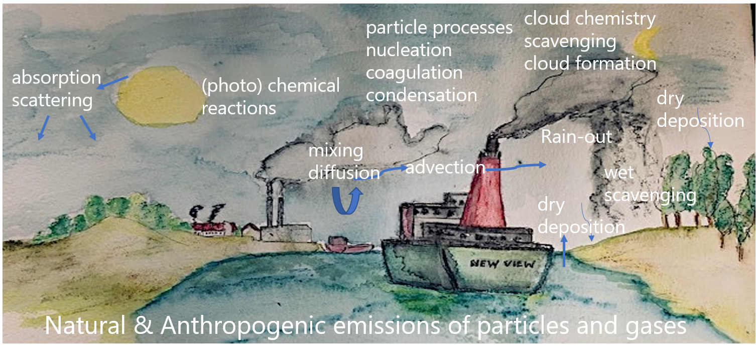
It is important to realize that air pollutants can have an impact on meteorology itself, by acting as a greenhouse gas, scattering or absorbing incoming light when in aerosol form, or be involved in the formation of clouds. This aspect will not be discussed here.
Meteorology is relevant for all aspects, ranging from mixing and transport to temperature or light dependent reaction rates and absorption of water. Depending on the removal rates, species may be removed with timescales of seconds, like heavy sand particles, to decades or longer, like halogen (Cl, Br)-containing gases, and be transported over ranges of a few meters to crossing the globe several times. Concentrations of gases are often expressed in volume mixing ratios (parts per billion, ppb) whereas for particulate matter the correct unit is in (micro)gram per cubic meter as there is no molecular weight associated to it. For ultrafine particles, concentrations are expressed as numbers of particles per cubic meter, for asbestos, the number of fibers per cubic meter is used.
Physical and chemical processes determining the properties of air pollutants
The properties of air pollutants, like solubility in water, attachment efficiencies to the Earth's surface (water, vegetation, soil) and size of particles, are key elements determining the lifetime and transport distances. These properties may change due to the interaction with other chemicals and with meteorology.
The main physical processes are:
- Condensation or evaporation with decreasing/increasing temperature. A potentially toxic aerosol may thus be covered by semi-volatile chemicals like ammonium sulfate, whilea gas may condensate on an aerosol and be transported further as part of this aerosol. Some pollutants exist at the same time in aerosol and in gas phase with their partitioning depending on air temperature and relative humidity.
- Gases may cluster to form ultrafine particles of a few nanometers (nucleation) that will grow to larger sizes.
- Particles may grow by coagulation: rapidly moving small particles bump into large slow-moving particles and remain attached to it.
- Particles may take up water (hygroscopicity), leading to a larger diameter.
Chemical conversions include:
- Chemical reactions between gas-phase pollutants and ambient gas, which alters the characteristics of an air pollutant or can lead to the formation of pollutants (e.g. NO2 being directly emitted by combustion, leading to ozone formation).
- Chemical reactions between aerosols and gases, often involving water attached to aerosol.
- Cloud droplets or water attached to aerosols have their own role in the chemistry of the atmosphere, and gases may diffuse into the water .
- Some pollutants may act as a catalyst.
- Some air pollutants may be degraded by (UV) light (photodegradation).
Pollutants are characterized by their chemical composition but for aerosols also the size distribution of particles is relevant. Note that the conservation of atoms always applies, but particle size distribution and particle number can be changed by physical processes. This has to be kept in mind when concentrations are expressed in particles per volume instead of mass concentrations.
Transport of air pollutants
Several processes determine the mixing and transport of chemicals in the air:
- Diffusion due to the motion of molecules, or Brownian motion of particles (random walk).
- Turbulent diffusion: the mixing due to (small-scale) turbulent eddies which have a random nature, but the strength of this diffusion is related to friction in the flow.
- Advection: the process of transport with the large-scale flow (wind speed and direction).
- Mixing or entrainment of different air masses leads to further mixing of air pollutants over a larger volume. This process is for example relevant when the sun rises, and air in the boundary layer is heated, rises, and mixes with the air in the layer above the boundary layer.
Although the processes of diffusion and transport are well-known, it is not an easy task to solve the equations describing these processes. For stationary point and line sources under idealized conditions, analytical descriptions can be derived in terms of a plume with concentration profile with a Gaussian distribution, but for more realistic descriptions the equations must be solved numerically. For complex flow around a building, computational fluid dynamics is required for an accurate description, for long-range transport a chemistry-transport model must be used.
Wet deposition
Wet deposition comprises the removal processes that involve water:
- Scavenging of particles by or dissolution of gases in cloud droplets. These cloud droplets may grow to larger size and rain out, thereby removing the dissolved air pollutants from the atmosphere (in-cloud scavenging).
- Particles below the clouds may be scavenged by falling raindrops (below-cloud scavenging).
- Occult deposition occurs when clouds are in contact with the surface (mountain areas) and cloud droplets containing air pollutants stick to the surface.
Wet deposition is a very efficient removal mechanism for both small (<0.1 µm diameter) and large aerosols (diameter >1 µm). Aerosols that are hygroscopic can grow in size by absorbing water, or shrink by evaporating water under dry conditions. This affects their deposition rate for wet or dry deposition.
Dry deposition
Dry deposition is partly determined by the gravitational forces on a particle. Heavy particles (≥ 5 µm) fall to the Earth's surface in a process called gravitational settling or sedimentation. In the lowest layer of the atmosphere, air pollutants can be brought close enough to the surface to stick to it or be taken up. In the turbulent boundary layer, air pollutants are brought close to the surface by the turbulent motion of the atmosphere, up to the very thin laminar layer (laminar resistance, only for gases) through which they diffuse to the surface. Aerosols or gases can stick to the Earth's surface or be taken up by vegetation, but they may also rebound. Several pathways take place in parallel or in series, similar to an electric circuit with several resistances in parallel and series. Therefore the resistance approach is often used to describe these processes.
Deposition above snow or ice is generally slow, since the atmosphere above it is often stably stratified with little turbulence (high aerodynamic resistance), the surface area to deposit on is relatively small (impactors) and aerosols may even rebound to an icy surface (collection efficiency of impactors) to which it is difficult to attach. On the other hand, forests often show high deposition velocities since they induce stronger turbulence in the lowermost atmosphere and have a large leaf surface that may take up gases by the stomata or provide sticking surfaces for aerosols. Deposition velocities thus depend on the type of surface, but also on the season, atmospheric stability (wind speed, cloud coverage) and ability of stomata to take up gases. When the atmosphere is very dry, for example, plants close their stomata and this pathway is temporarily shut down. For particles, the dry deposition velocity is lowest at sizes of 0.1-1 µm.
Re-emission
Once air pollutants are removed from the atmosphere, they can be part of the soil or water compartments which can act as a reservoir. This is in general only taken into account for a limited number of chemicals. Ammonia or persistent organic pollutants may be re-emitted from the soil by evaporation. Dusty material or pollutants attached to dust may be brought back into the atmosphere by the action of wind. This is relevant for bare areas like agricultural lands in wintertime, but also for passing vehicles that bring up the dust on a road by the flow they induce.
Atmospheric fate modelling
Due to the many relevant processes and interactions, the fate of chemical pollutants in the air has to be determined by using models that cover the most important processes. Which processes need to be covered depends on the case study: a good description of a plume of toxic material during an accident, where high concentrations, strong gradients and short timescales are important, requires a different approach than the chronic small release of a factory. Since it would require too heavy numerical simulations to include all aspects, one has to select the relevant processes to be included. Key input for all transport models are emission rates and meteorological input.
When one is interested in concentrations close to a specific source, next to emission rate the effective emission height is important, and processes that determine dispersion: wind speed, atmospheric stability. Chemical reaction rates and deposition velocities should be included when the time horizon is long or when the reactions are fast or deposition velocities are high.
When one is interested in actual concentrations resulting from releases of multiple sources and species over a large area of interest, like for an air quality forecast, the processes of advection, deposition and chemical conversions become more relevant, and input meteorology needs to be known over the area. Sharp gradients close to the individual sources are, however, no longer resolved. In particular rain can be a very efficient removal mechanism, removing most of the aerosol within one hour. Dry deposition is slower, but results in a lifetime of less than a week and transport distances of less than 1,000 km for most aerosols. For some gaseous compounds like halogens and N2O deposition does hardly play a role and they are chemically inert in the troposphere, leading to very long lifetimes.
To assess the overall long-term fate of a new chemical to be released to the market, the potential concentrations in air, water and soil have to be determined. Ideally, models for air, soil and water are used together in a consistent way, including their interaction For many air pollutants the atmospheric lifetime is short but determines where and in which form they are deposited onto ground and water surfaces, where they may accumulate. This means that even if a concentration in air is relatively low at a certain distance from a source, the deposition of an air pollutant over a year may still be significant. Figure 2 shows an example of annual mean modelled concentrations and annual total deposition of a hypothetical passive (non-reactive) soot-like tracer that is released at 1 kg/hour at a fictitious site in The Netherlands. Annual mean concentrations are small compared to ambient concentrations of particulate matter, but the footprint of the accumulated deposition is larger than that of the mean concentration, since the surface acts as a reservoir. This implies that re-emission to air can be relevant. It may take several years for soil or water before an equilibrium concentration is reached in these compartments from the deposition input, as different processes and time scales apply. Mountain ranges are visible in the accumulated wet deposition (Alps, Pyrenees), as they are areas with enhanced precipitations.
In addition to spatially explicit modelling, also box models exist that have the advantage that they can make long-term calculations for a continuous release of a species, including interaction between the compartments air, soil and water. They can be used to determine when an equilibrium concentration is reached within a compartment, but these models cannot resolve horizontal concentration gradients within a compartment.
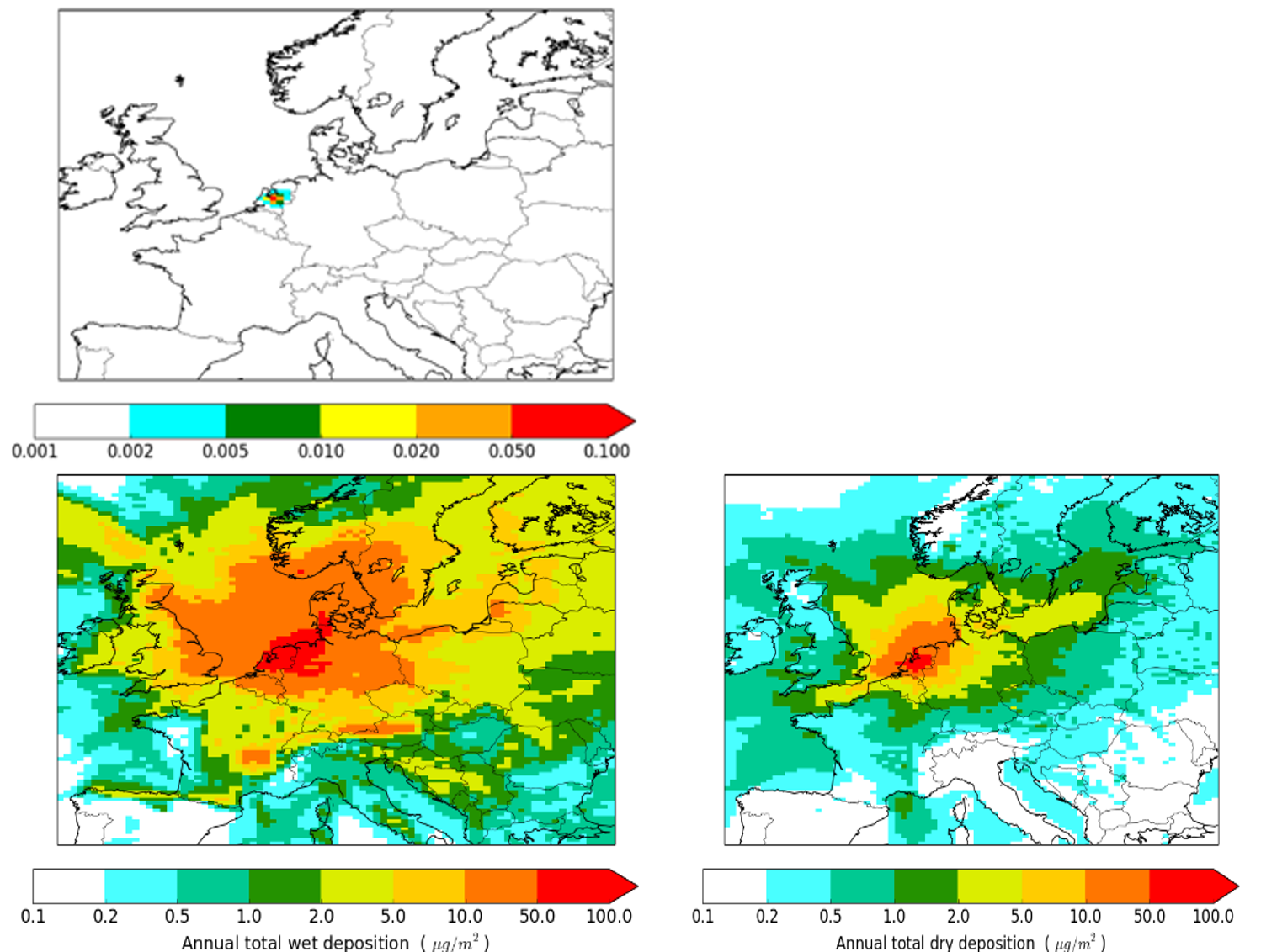
Figure 2. Constant release of a passive tracer from a point source in The Netherlands. Upper panel shows the annual mean concentration, the lower panel shows the accumulated wet and dry deposition over one year. Note the nonlinear colour scale to cover the large range of values. Source: https://doi.org/10.3390/atmos8050084.
Learn more
EU air quality, policy and air quality legislation: http://ec.europa.eu/environment/air/index_en.htm
US hazardous air pollutants, including lists of toxics: https://www.epa.gov/haps
Plume dispersion approach: http://courses.washington.edu/cewa567/Plumes.PDF
Chemistry-transport models: www.narsto.org/sites/narsto-dev.ornl.gov/files/Ch71.3MB.pdF
Seinfeld, J., Pandis, S.N. Atmospheric Chemistry and Physics, from air pollution to climate change, Wiley, 2016, covering all aspects.
John, A. C., Küpper, M., Manders-Groot, A. M., Debray, B., Lacome, J. M., Kuhlbusch, T. A. (2017). Emissions and possible environmental implication of engineered nanomaterials (ENMs) in the atmosphere. Atmosphere, 8(5), 84.
Which processes determine the concentration of a pollutant in the air very close to its point of emission?
When fine particles (<1µm diameter) are released in the lowest 100 m of the atmosphere, how far will they be transported? And what processes do contribute to removal of the particles from the air?
When gases are released in the lowest 100 m of the atmosphere, how far do they get?
3.1.3. Hydrosphere
Authors: John Parsons
Reviewers: Steven Droge, Sean Comber
Leaning objectives:
You should be able to:
- describe the most important chemical components and their sources
- describe the most important chemical processes in fresh and marine water.
- be familiar with the processes regulating the pH of surface water.
Keywords: Hydrogen bonding, carbonates, dissolved salts
The properties and importance of water
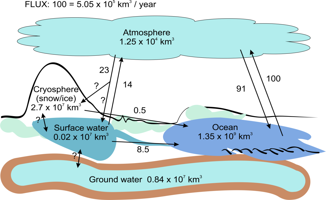
Water covers 71% of the earth's surface and this water, together with the smaller amounts present as gas in the atmosphere, as groundwater and as ice is referred to collectively as the hydrosphere. The bulk of this water is salt water in the oceans and seas with only a minor part of freshwater being present as lakes and rivers (Figure 1).
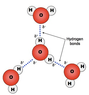
Water is essential for life and also plays a key role in many other chemical and physical processes, such as the weathering of minerals and soil formation and in regulating the Earth's climate. These important roles of water derive from its structure as a small but very polar molecule arising from the polarised hydrogen-oxygen bonds (Figure 2). As a consequence, water molecules are strongly attracted by hydrogen bonding, giving it relatively high melting and boiling points, heat capacity, surface tension, etc. The polarity of the water molecule also makes water an excellent solvent for a wide variety of ionic and polar chemicals but a poor solvent for large nonpolar molecules.
The freshwater environment
As mentioned above, freshwater is only very small proportion of total amount of water on the planet and most of this is present as ice. Since this water is in contact with the atmosphere and the soils and bedrock of the Earth's crust, it dissolves both atmospheric gases such as oxygen and carbon dioxide and salts and organic chemicals from the crust. If we compare the relative compositions of cations in the Earth's crust and the major dissolved species (Table 1) it is clear that these are very different. This difference reflects the importance of the solubility of these components. For ionic chemicals, this depends on both their charge and their size (expressed as z/r2, where z is the charge and r the radius of an ion). As well as reflecting the properties of the local crust, the composition of salts is also influenced by precipitation and evaporation and the deposition of sea salt in coastal regions.
Table 1. Comparison of the major cation composition of average upper continental crust and average river water. (*except aluminum and iron from Broecker and Peng (1982))
|
Upper continental crust (mg/kg) (Wedepohl 1995*) |
River water (mg/kg) |
|
|
Al |
77.4 |
0.05 |
|
Fe |
30.9 |
0.04 |
|
Ca |
29.4 |
13.4 |
|
Na |
25.7 |
5.2 |
|
K |
28.6 |
1.3 |
|
Mg |
13.5 |
3.4 |
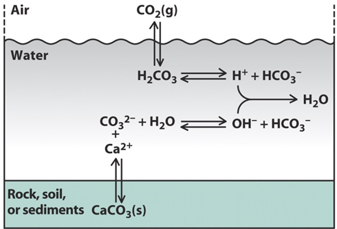
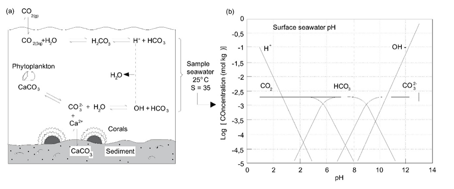
The pH of surface water is determined by both the dissolution of carbonate minerals and carbon dioxide from the atmosphere. These components are part of the set of equilibrium reactions known as the carbonate system (Figure 3).
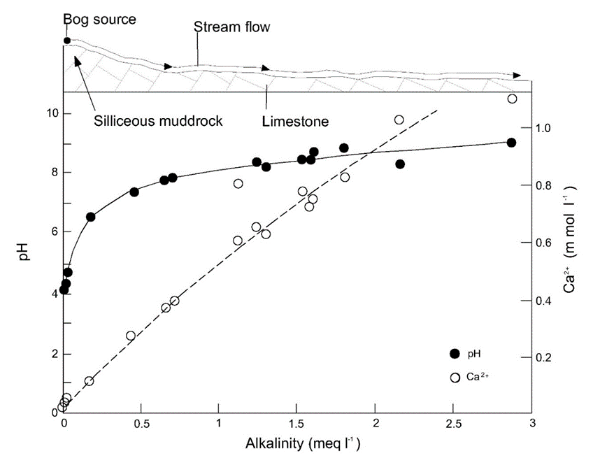
At equilibrium with the current atmospheric CO2 concentration and solid calcium carbonate, the pH of surface water is between 7 and 9 but this may reach more acidic values where soils are calcium carbonate (limestone) poor. This is illustrated by the pH values measured in a river in Northern England, where acidic, organic carbon-rich water at the source is gradually neutralised once the river encounters limestone rich bedrock (Figure 4).
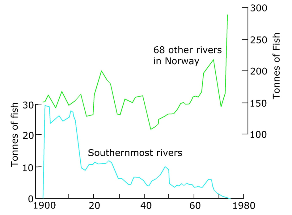
As well as these natural processes, there are human influences on the pH of surface water including acidic precipitation resulting from fossil fuel combustion and acidic effluents from mining activities caused by oxidation and dissolution of mineral sulphides. Regions such as Southern Scandinavia with carbonate-poor soils are particularly vulnerable to acidification due to these influences and this is reflected in for example, reduced fish populations in these vulnerable regions (see Figure 5). More recently, reduced coal burning and the decline in heavy industry is resulting in the recovery of pH values in upland areas across Europe.
Dissolved oxygen is of course essential to aquatic life and concentrations are in general adequate in well mixed water bodies. Oxygen can become limiting in deep lakes where thermal stratification restricts the transport of oxygen to deeper layers, or in water bodies with high rates of organic matter decomposition. This may result in anoxic conditions with significant ecological impacts and on the behaviour of chemical contaminants.
The marine environment
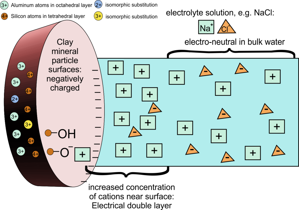
Freshwater eventually moves into seas and oceans where the concentrations of dissolved species are much higher than in the freshwater environment. This is partly due to the effects of evaporation of water from the oceans but is also be due to specific marine sources of some dissolved components. Estuaries are the transition zones where freshwater and seawater mix. These are highly productive environments where increasing salinity has a major impact on the behaviour of many chemicals, for example on the speciation of metals and the aggregation of colloids as a result of cations shielding the negative surface change of colloidal particles (Figure 6). Increasing salinity also affects organic chemicals, with ionic chemicals forming ion pairs, and even reducing the solubility of neutral organics (the so-called salting-out effect). As well as these chemical effects due to increasing salinity, the lowering of flow rates in estuaries leads to the deposition of suspended particles.
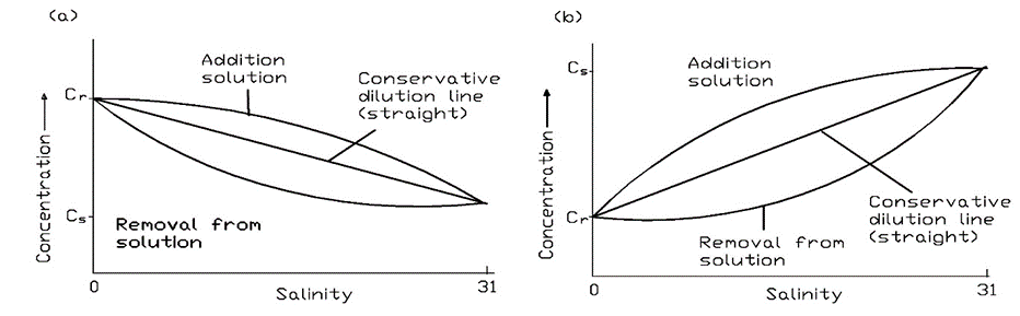
Since the concentrations of pollutants are in general lower in the marine environment than in the freshwater environment, concentrations in estuaries decrease as freshwater is diluted with seawater. Measuring salinity at different locations in estuaries is a convenient way to determine the extent of this dilution. Components that are present in higher concentrations in seawater will of course show an increase with salinity unless. Plotting salinity against the concentrations of chemicals at different locations can yield information on whether they behave conservatively (i.e. only undergoing mixing) or are removed by processes such as degradation or partitioning into the atmosphere or sediments. Figure 7 shows examples of plots expected for conservative chemicals and those that are either removed in the estuary or have local sources there. Models describing the behaviour of chemicals in estuaries can be used with these data to derive the rates of removal or addition of the chemical in the system.
The open ocean is sufficiently mixed for the composition of major dissolved constituents to be fairly constant, except in local situations as a result of upwelling of deep nutrient-rich waters or the biological uptake of nutrients. In coastal regions the concentrations of chemicals and other components originating from terrestrial sources may also be locally higher. The major components in seawater are listed in Table 2 with their typical concentrations.
Table 2. Major ion composition of freshwater and seawater.
|
Seawater (mmol/L) (Broecker and Peng, 1982) |
River water (mmol/L) |
|
|
Na+ |
470 |
0.23 |
|
Mg2+ |
53 |
0.14 |
|
K+ |
10 |
0.03 |
|
Ca2+ |
10 |
0.33 |
|
HCO3- |
2 |
0.85 |
|
SO42- |
28 |
0.09 |
|
Cl- |
550 |
0.16 |
|
Si |
0.1 |
0.16 |
These concentrations may be higher in waterbodies that are partly or wholly isolated from the oceans and are impacted by evaporative losses of water (e.g. Mediterranean, Baltic, Black Sea). In extreme case, concentrations of salts may exceed their solubility product, resulting in precipitation of salts in evaporate deposits.
As is the case in freshwater, carbonates play an important role in regulating the ocean pH. The fact that the oceans are supersaturated in calcium carbonate makes it possible for a variety of organisms to have calcium carbonate shells and other structures. The important processes and equilibria involved are illustrated in Figure 8. There is concern that one of the most important effects of increasing atmospheric carbon dioxide will be lowering of ocean pH to values that will result in destabilisation of these carbonate structures.
References
Andrews, J.E., Brimblecombe, P., Jicketts, T.D., Liss, P.S., Reid, B.J. (2004). An Introduction To Environmental Chemistry, Blackwell Publishers, ISBN 0-632-05905-2.
Baird, C., Cann, M. (2012). Environmental Chemistry, Fifth Edition, W.H. Freeman and Company, ISBN 978-1429277044.
Berner, E.K., Berner, R.A. (1987). Global water cycle: geochemistry and environment, Prentice-Hall.
Broecker, W.S., Peng, T.S. (1982). Tracers in the Sea, Lamont-Doherty Geol. Obs. Publ.
Henriksen, A., Lien, L., Rosseland, B.O., Traaen, T.S., Sevaldrud, I.S. (1989). Lake Acidification in Norway: Present and Predicted Fish Status. Ambio 18, 314-321
Wedepohl, K.H. (1995). The composition of the continental crust, Geochimica Cosmochimica Acta 59, 1217-1232.
The concentrations of dissolved salts in rivers and lakes is determined by three processes. Describe these processes and the characteristic composition of waterbodies where one of these processes is dominant.
In addition to the well-known effects on global climate, increasing atmospheric CO2 is also expected to have an impact on the pH of the oceans. Which processes are responsible for determining the pH of the oceans?
How could increasing atmospheric CO2 affect these processes?
What effects could increasing acidity of the oceans have on marine organisms?
3.1.4. Sediment
In preparation
3.1.5. Soil
Author: Kees van Gestel
Reviewers: John Parsons, Jose Alvarez Rogel
Learning goals
You should be able to
- describe the main components of which soils consist
- describe how soil composition influences properties that may affect the fate of chemicals in soil
Keywords:
Particle size distribution, Porosity, Minerals, Organic matter, Cation Exchange Capacity, Water Holding Capacity
Introduction
Soil is the upper layer of the terrestrial environment that serves as a habitat for organisms and medium for plant growth. In addition, it also plays an important role in water storage and purification and helps to regulate the Earth's atmosphere (e.g. carbon storage, gas fluxes, …).
Soils are composed of three phases (Figure 1).
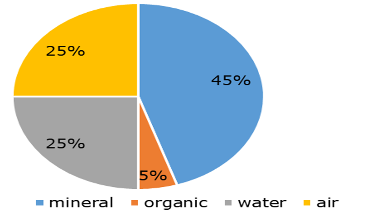
The solid phase is formed by mineral and organic components. Mineral components appear in different particle sizes from coarse particles (sand), intermediate (silt) and fine (clay) which combination determine soil texture. The particles can be arranged to form porous aggregates; soil pores being filled with air and/or water. The proportion of air in soils depends on soil moisture content. The composition of the soil solid phase may be quite variable.
The gaseous phase has a similar composition as the air, but due to the respiration of plant roots and the metabolic activity of soil microorganisms, O2 content generally is lower and CO2 content higher. Exchange of gases between soil pores and atmospheric air takes place by diffusion. Diffusion proceeds faster in dry soil and much slower when soil pores are filled with water.
The liquid phase of the soil, the soil solution or pore water, is an aqueous solution containing ions (mainly Na+, K+, Ca2+, Cl-, NO3-, SO42-, HCO3-) from dissolution of a variety of salts, and also contains dissolved organic carbon (DOC, also referred to as dissolved organic matter, DOM). The soil solution is part of the hydrological cycle, which involves input from among others rain and irrigation, and output by water uptake by plants, evaporation, and drainage to ground and surface water. The soil solution acts as a carrier for the transport of chemicals in soil, both to plant roots, soil microorganisms and soil animals and to ground and surface water.
Soil solids
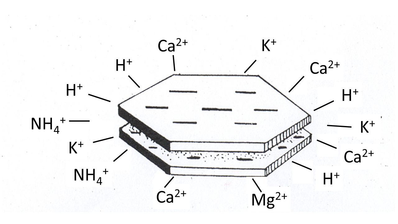
The soil solid phase consists of mineral and organic soil particles. Based on their size, the mineral particles are divided into sand (63-2000 µm), silt (2- 63 µm), and clay (<2 µm). With increasing particle size, the specific surface area decreases, pore size increases and water retention capacity decreases. The sand fraction mainly consists of quartz (SiO2) and does not have any sorption properties because the quartz crystals are electrically neutral. Sandy soils have large pores, so a low capacity to retain water. In soils with a high silt fraction, smaller pores are better represented, giving these soils a higher water retention capacity. Also the silt fraction has no adsorptive properties. Clays are aluminium silicates, lattices composed of SiO4 tetrahedrons and Al(OH)6 octahedrons. Upon the formation of clay particles, isomorphic substitution occurred, a process in which Si4+ was replaced by Al3+, and Al3+ by Mg2+. Although having similar diameters, these elements have different valences. As a consequence, clay particles have a negative charge, making positive ions to accumulate on their surface. This includes ions important for plant growth, like NH4+, K+, Na+ and Mg2+, but also cationic metals (Figure 2). Many other minerals have pH-dependent charges (either positive or negative) which are also important in binding cations and anions.
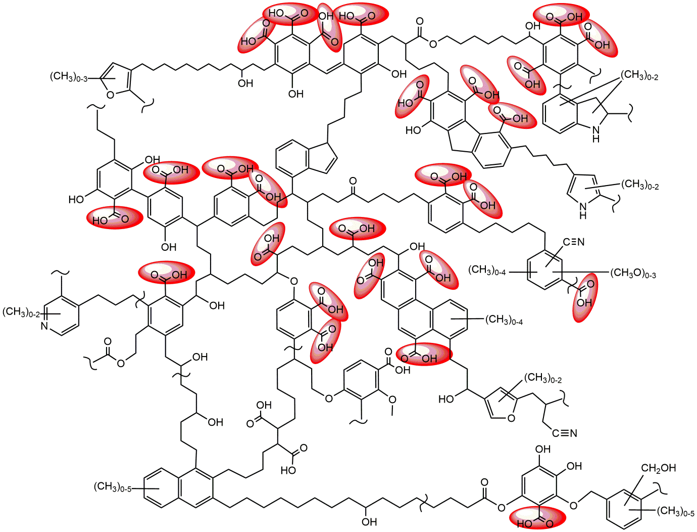
In addition to mineral particles, soils also contain organic matter, which includes all dead plant and animals remains and their degradation products. Living biota is not included in the soil organic matter faction. Organic matter is often divided into: 1. humin, non-dissolved organic matter associated with clay and silt particles, 2. humic acids having a high degree of polymerization, and 3. fulvic acids containing more phenolic and carboxylic acid groups. Humic and fulvic acids are water soluble but their solubility depends on pH. For example, humic acids are soluble at alkaline pH but not at acidic pH. The dissociation of the phenolic and carboxylic groups gives the organic matter also a negative charge (Figure 3), the density of which increases with increasing soil pH. The soil organic matter acts as a reservoir of nitrogen and other elements, provides adsorption site for cations and organic chemicals, and supports the building of soil aggregates and the development of soil structure.
The binding of cations to the negatively charged sites on the soil particles is an exchange process. The degree of cation accumulation near soil particles depends on their charge density, the affinity of the cations to the charged surfaces (which is higher for bivalent than for monovalent cations), the concentration of ions in solution (the higher the concentration of a cation in solution, the higher attraction to soil particles), etc. Due to their binding to charged soil particles, cations are less available for leaching and for uptake by organisms. The Cation Exchange Capacity (CEC) is commonly used as a measure of the number of sites available for the sorption of cations. CEC is usually expressed as cmolc/kg dry soil. Soils with higher CEC have a higher capacity to bind cations, so cationic metals show a lower (bio)availability in high CEC soils (see the Section on metal speciation). CEC depends on the content and type of clay minerals, with montmorillonite having a higher CEC than e.g. kaolinite, organic matter content and pH of the soil. In addition to clay and organic matter, also aluminium and iron oxides and hydroxides may contribute to the binding of cations to the soil.
Soil water
The transport of water through soil pores is controlled by gravity, and by suction gradients which are the result of water retention by capillary and osmotic processes. Capillary binding of water is stronger in smaller soil pores, which explains why clayey soils have higher water retention capacities than sandy soils. The osmotic binding of water increases with increasing ionic strength, and is especially high close to charged soil particles like clay and organic matter where ions tend to accumulate.
The stronger water is retained by soil, the lower its availability is for plants and other organisms. The strength by which water is retained depends on moisture content, because 1. at decreasing moisture content the ionic strength of the soil solution and therefore osmotic binding increases, 2. when soil moisture content decreases the larger soil pores will be emptied first, leading to increasing capillary retention of the remaining water in smaller pores. Water retention curves describe the strength with which water is retained as a function of total water content and in dependence of the composition of the soil. Figure 4 shows pF curves for three different soil types.
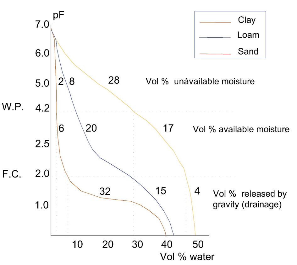
A pF value of 2.2-2.5 corresponds with a binding strength of 200 to 300 hPa. This is called field capacity; water is readily available for plant uptake. At pF 4.2 (15,000 hPa), water is strongly bound in the soil and no longer available for plant uptake; this is called the wilting point. For soil organisms, not the total water content of a soil is of importance but rather the content of available water. Water retention curves may be important to describe the availability of water in soil. Toxicity tests with soil organisms are typically performed at 40-60% of the water holding capacity (WHC) of the soil, which corresponds with field capacity.
References/further reading
Schulten, H.-R., Schnitzer, M. (1997). Chemical model structure for soil organic matter and soils. Soil Science 162, 115-130.
Blume, H.-P., Brümmer, G.W., Fleige, H., Horn, R., Kandeler, E., Kögel-Knabner, I., Kretzschmar, R., Stahr, K., Wilke, B.-M. (2016). Scheffer/Schachtschabel Soil Science, Springer, ISBN 978-3-642-30941-0
What are the main components of the solid phase of a soil?
When considering two different soils, a sandy and a clayey soil, which one has the highest available volume of water when both soils have the same total water content? Explain your answer.
What is the agricultural and environmental importance of the cation exchange capacity of soils?
Explain the role of clay minerals and organic matter in the retention of cationic metals in soils.
Which two factors explain the fact that the availability of cationic metals increases with decreasing soil pH?
3.1.6. Groundwater
(draft)
Author: Thilo Behrends
Reviewer: Steven Droge, John Parsons
Leaning objectives:
You should be able to:
- understand the significance of redox reactions for the fate of potentially toxic compounds in groundwaters and aquifers.
- apply the Nernst equation to assess the feasibility of redox reactions.
Keywords: Aquifer, Nernst equation, electron transfer, redox potential, half reactions
Introduction
Some definitions conceive all water beneath the earth's surface as groundwater while others restrict the definition to water in the saturated zone. In the saturated zone the pores are completely filled with water in contrast to the undersaturated zone in which some pores are filled with gas and capillary action are important for moving water. Geological formations, which host groundwater in the saturated zone, can be classified as 'aquifer', ' aquitard', or 'aquifuge' depending on their permeability. In contrast to aquitard and aquifuge, which have a low permeability, an aquifer permits water to move in significant rates under ordinary field conditions. Aquifers typically have a high porosity and the pores are well connected with each other. Examples of aquifers include sedimentary layers of sand or gravel, carbonate rocks, sandstones, volcanic rocks and fractured igneous rocks. The redox chemistry discussed in this chapter is focusing on aquifers in sedimentary formations.
Groundwaters are an important source for drinking water and the quality of groundwater is, therefore, of high importance for protecting human health. However, aquifers also represent a habitat for bacteria and aquatic invertebrates and are, therefore, also an object for ecotoxicological studies. Furthermore, groundwater can act as a transportation pathway connecting different environmental compartments e.g. soils with rivers or oceans. Groundwater thus plays a role in the distribution of contaminants in the environment.
Transport of contaminants in aquifers
The movement of a chemical in groundwater is controlled by three processes: advection, dispersion and reaction. Advection is the transport of a chemical in dissolved form together with the groundwater flow. When a chemical is released from a point source into groundwater with a constant flow direction, a plume is forming downstream of the source. The spreading of the chemical is due to dispersion. There are two reasons for this spreading: First, molecular diffusion causes transport of the chemical independently from advection; Second, differences in groundwater velocities at different scales causes mixing of the groundwater (mechanical dispersion) in the direction of groundwater flow but also perpendicular to it. Several process can retard the transport of chemicals or can cause its removal from the system (e.g. degradation). For the mobility of a chemical, the distribution between immobile solid phase and moving liquid phase is of key importance in groundwater (see chapter 3.4). There are several processes which can lead to the degradation of a compound in aquifers. Microbial activity can contribute to the degradation of chemicals but also abiotic reactions can be of importance. For some chemical, redox reactions are relevant which are discussed in the following section.
Redox reactions in aquifers
Many elements are redox-sensitive under environmental conditions. This means they occur naturally in different 'redox states'. For example oxidation or reduction of carbon plays a pivotal role in the energy metabolism of living organisms and carbon occurs in oxidation states from +IV in CO2 (because the two oxygen atoms both count as -II ((because oxygen is more electronegative than carbon)), and the total molecule should balance out) to -IV in CH4 (because each H-atom counts as +I ((because hydrogen is less electronegative than carbon))). Also potentially toxic elements, such as arsenic, are found in nature in different oxidation states. Important oxidation states of arsenic are +V, (e.g. AsO43-, arsenate), + III (e.g. AsO3-3, arsenite), 0 (elemental arsenic or arsenic associated with sulfide as in FeAsS, arsenopyrite). Arsenic can also have negative oxidation states when it forms arsenides such as FeAs2 (löllingite). Bioavailability, toxicity and mobility of redox sensitive elements are usually strongly dependent on their oxidation state. For example, arsenite tends to be more toxic and more mobile than arsenate. For this reason, assessing the redox state of potentially toxic elements is an important element of environmental risk assessment of groundwater.
Organic contaminants can also undergo redox transformations. At the earth surface, when oxygen is present, (photo-)oxidation is an important degradation pathway for organic contaminants. In subsurface environments, when oxygen concentrations are often very low (anoxic conditions), reduction can play an important role in degradation pathways. For example, the reductive dehalogenation of chlorinated hydrocarbons or the reduction of nitroaromatic compounds have been extensively investigated. The reduction of these compounds can be mediated by microorganisms but they can also occur abiotically on solid surfaces present in the subsurface. In any case, reduction of organic contaminants is only possible when the reaction is thermodynamically feasible. For this reason it is necessary to know the redox conditions in, for example, an aquifer.
Quantitative assessment of redox reactions
As the name indicates, redox reactions combine oxidation of one constituent in the system with the reduction of another and, hence, involve electron transfer. The oxidation of arsenite with elemental oxygen to arsenate has following stoichiometry:

It is important that the stoichiometries of redox reactions are not only charge- and mass-balanced but also electron-balanced. Here, arsenic releases two electrons when going from oxidation state +III to +V (arsenite becomes oxidized to arsenate) while one oxygen atom takes up the two electrons and goes from oxidation state 0 to -II (elemental oxygen becomes reduced). For this reaction an equilibrium constant can be obtained and based on the activities (or concentrations) of dissolved reactants and products it can be evaluated whether the reaction is in equilibrium or in which direction the reaction is thermodynamically favorable.
When a natural system contains several different redox-active constituents, a large number of possible redox reactions can be formulated and evaluated separately. In this situation it is more convenient to formulate and compare half reactions. For examples, the oxidation of arsenite with oxygen can be split up into the reactions of arsenic and oxygen.


Half reactions are typically formulated as reduction reactions (electrons are on the left hand side of the reaction). The Eho is the standard redox potential and represents the electrical potential, which would be measured in a standardized electrochemical cell which contains on one side, H3AsO4, H3AsO3 and H+, all with activities of 1 mol l-1, and a solution containing 1 mol l-1 H+ in equilibrium with H2 gas with a pressure of 1 bar, on the other side.
In natural environments the pH is usually not 0 and the activities of arsenite and arsenate are not 1 mol l-1. The redox potential, Eh under these conditions can be calculated using the Nernst equation:

where:
R is the ideal gas constant ( 8.314 J mol-1 K-1),
T the temperature in K,
z is the number of electrons which are transferred in the reaction,
F the Faraday constant (96485 mol C-1).
In the ratio ox/red, 'ox' represents the activities or pressures of the constituents on the right hand side of the half reaction, whereby the stoichiometric factor becomes the corresponding exponent, while 'red' represents the right hand side of the half reaction.
The redox potentials of different half reactions can be compared:
- The half reaction with the higher redox potential provides the electron acceptor in the thermodynamically favorable redox reaction,
- The half reaction with the lower potential provides the electron donor.
In other words, it is thermodynamically favorable that the half reaction with the high potential proceeds from left to right and the half reaction with the low potential from right to left.
Redox conditions in aquifers
The redox conditions in an aquifer depends on the inherited inventory of oxidants and reductants during the formation of the geological formation and the processes which have been occurring throughout its history. Oxidants and reductants can have entered the aquifer by diffusion or with the infiltrating water and slowly progressing redox reaction can have modified the assemblage of oxidants and reductants. In the absence of (microbial) catalysis redox reactions often have very slow kinetics. Furthermore, due to photosynthesis, redox reactions are not in equilibrium at the earth's surface and the upper part of the underlying subsurface. As a consequence, the redox conditions in an aquifer can usually not be represented in one unique redox potential. This implies that values obtained for groundwaters with electrochemical measurements, e.g. potentiometric measurements using redox electrodes, might be not representative for the redox conditions in the aquifer. Furthermore, relevant half reactions in the aquifer often involve solids (heterogeneous reactions) with low solubility, implying that the concentrations in solution (for example of Fe3+) are too low to be detected. Hence, evaluating the redox conditions in subsurface environments is often challenging.
Oxygen concentrations in groundwaters are often virtually zero, as oxygen in infiltrating rain water or entering the subsurface by molecular diffusion is often consumed before it can reach the aquifer. Hence, 'reducing conditions' typically prevail in aquifers. The redox potential measured in a system may reflect the dominant electron acceptors besides oxygen that are present in the system (Figure 1).
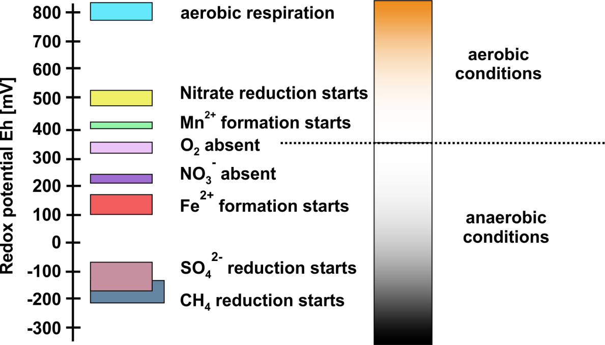
In sediments or sedimentary rocks, redox reactions after deposition are predominately driven by the oxidation of organic matter, which entered the sediment during its deposition. However, the aquifer might also have received dissolved organic matter via infiltrating water. The oxidation of organic matter is predominately microbially mediated and predominately coupled to the reduction of elemental oxygen (if present). However, when elemental oxygen is depleted, which is usually the case, other electron acceptors are used by microorganisms. Relevant electron acceptors (see Figure 1) in anoxic environments include:
- Nitrate (in dissolved form),
- Mn(IV) (as solid surface),
- Mn(III) (as solid surface),
- Fe(III) (as solid surface),
- Sulphate (in dissolved form).
Nitrate and sulphate can be present in dissolved form while Mn(IV), Mn(III), Fe(III) occur as solids with low solubility. The (hydr)oxide solids of these metals, such as goethite (FeOOH) or manganite (MnOOH) are mostly accessible for microbial reduction while Mn(III) or Fe(III) in silicates can only be partially reduced or are not bioavailable for reduction. When also these electron acceptors run short, methanogenesis can be initiated.
Microorganisms, which reduce sulphate, Mn or Fe(III), can use the products of fermentative organisms. These fermentative organisms produce short-chain fatty acids, such as acetate or lactate, but often also release hydrogen gas. That is, hydrogen concentrations in groundwater reflect a steady state of hydrogen production and consumption, and are typically limited by the rates of production. As a consequence, hydrogen concentrations in groundwater are often at the physiological limit of the consuming organism. The concentrations are just sufficient to allow the organism to conserve energy from oxidizing the hydrogen. This limit increases according to the sequence of electron acceptors (Figure 1): nitrate reduction < Mn reduction < Fe reduction < sulphate reduction < methanogenesis when the corresponding compounds are present in relevant amounts or concentrations. For this reason, concentrations of dissolved hydrogen can be a useful indicator to identify the dominant, anaerobic respiration pathway in an aquifer. For example, one can determine whether sulphate reduction is enabled or methanogenesis has set in. The hydrogen concentrations in the groundwater can also directly be used to assess whether the microbial reduction of metals, metalloids, chlorinated hydrocarbons, nitro aromatic compounds or other organic contaminants is feasible.
The reduction of Fe(III)(hydr)oxides are sulphate leads to the formation of Fe(II) and sulphide, which, in turn, typically results in the precipitation of ferrous solids such as FeCO3 (siderite), FeS (mackinawite) or FeS2 (pyrite). These Fe(II) containing minerals often play an important role in the abiotic reduction of organic or inorganic contaminants in aquifers. When the composition of the groundwater and the mineral assemblage is known, the Nernst equation can be used to calculate the redox potential of relevant half reactions in the aquifer. These redox potential can be then used for evaluating whether reduction of potentially toxic compounds is possible or not. For example, the half reaction for the reduction of an amorphous ferric iron hydroxide coupled to the precipitation of siderite is given by:


At given pH and carbonic acid concentration, the corresponding redox potential can be calculated using the Nernst equation. This redox potential can be compared to that obtained from the Nernst equation for the reductive dichlorination of tetrachloroethylene (Cl2C=CCl2)


With this approach the feasibility of redox reactions involving potentially organic and inorganic compounds can be evaluated in aquifers. That does, however, not imply that the corresponding reactions also occur within the relevant time scale. For this the kinetics of the reaction have to be known and have been studied for many reactions of potential relevance in aquifer systems. However, the kinetics of redox reactions are not subject of this section.
References
Sparks, D. (2002). Environmental Soil Chemistry, Second Edition, Academic Press, Chapters 5 and 8, ISBN 978-0126564464.
Essington, M.E. (2004). Soil and Water Chemistry: An Integrative Approach, Chapters 7 and 9, CRC Press, ISBN 978-0849312588
Which processes control the movement of chemicals in groundwater? Define each of these processes.
Redox reactions of contaminants in groundwater are controlled by the redox potential. What are the most important chemicals and processes determining the redox potential?
How can the redox potential in aquifer be determined? What are the disadvantages of these methods?
3.1.7. Biota
(draft)
Author: Steven Droge,
Reviewer: Nico van der Brink, John Parsons
Leaning objectives:
You should be able to:
- explain the effect of cell and body composition on toxicokinetics of compounds
- describe the role of biota in the environmental fate of chemicals
Keywords: cellular composition, body composition, exposure routes, absorption, distribution
Introduction
Just like soil, water, and air, the organic tissue of living organisms can also be regarded as a compartment of the ecosystem where chemical pollutants can accumulate or can be broken down. The internal concentration in living organisms provide important information on chemical exposure and ultimately determines the environmental risk of pollution, but it is important to understand the key features of tissue that influence chemical partitioning into organisms. Chemical accumulation in the tissue of living organisms is a series of chemical and biological processes, briefly based on:
- chemical uptake (mostly permeation from bulk media over certain membranes into cells);
- internal distribution (e.g. via blood flows through organs);
- metabolism (e.g. biotransformation processes in for instance the liver).
- excretion (e.g. through urine and feces, but also via gills, sweat, milk, or hairs)
These four processes are the basis of toxicokinetic modeling, and are often summarized as Absorption, Distribution, Metabolism, and Excretion, or "ADME". These ADME processes can strongly vary for different polluting compounds due to the properties of the chemical structure. These ADME processes can also strongly vary for different organisms, because of:
- the physiological characteristics (e.g. having gills, lungs, or roots, availability of specific chemical uptake mechanisms, presence of specific metabolic enzymes, size-related properties like metabolic rate),
- the position in the polluted environment (flying birds or midge larvae living in sediment),
- the interaction with the polluted environment (living in soil or water, food choice, etc.)
- the behaviour in the polluted environment (being sessile or able to move (temporarily) away from a polluted spot).
More details of these toxicokinetic processes are presented in section 4.1 on Toxicokinetics and bioaccumulation. The current module aims to provide a summary of the key features of different tissue components that explain the internal distribution of chemicals (distribution), the different types of contact between pollutants and organisms (exposure-absorption), and temporal changes in physiology that may affect internal exposure (e.g. excretion, which includes examples such as release of POPs via lactation, and increasing POP concentrations during starvation). Before we discuss how chemicals are taken up into biota, it is important to first define the key chemical properties and the molecular composition of tissue that influence the way chemicals are absorbed from the surrounding environment and distributed throughout an organism.
Absorption-distribution: Tissue building blocks
All organisms are composed of cells, which are composed of a cell membrane, surrounding the largely watery solution filled with inner organelle membranes, protein structures, and DNA/RNA. Prokaryote organisms such as bacteria, but also algae, fungi and plants have reinforced membranes with cell walls to prevent water leaking by high osmotic pressures, and to protect the cell membrane. Metabolic energy is stored in large molecules such as fatty esters and sugars. Remarkably, for all existing living organism species, these tissue components are mostly structures made out of relatively simple and repetitive molecular building blocks, with minor variations on side chains. See examples in Figure 1. The composition of organs, as a collection of specific cells, in terms of the percentage of lipids, proteins and carbohydrates is important for the overall toxicokinetics of chemicals in the whole organism.
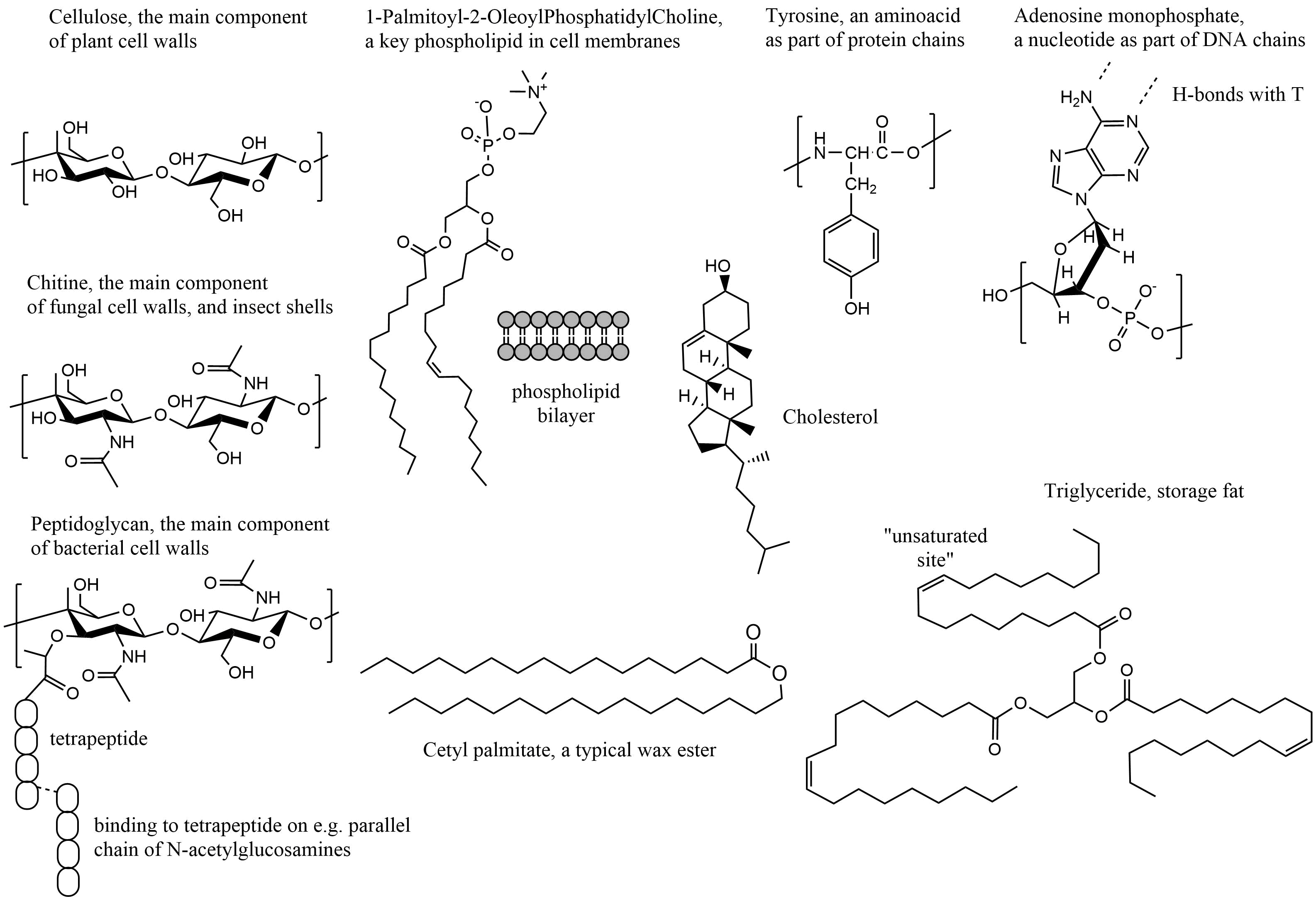
Cell walls are mostly made from highly polar polysaccharides, e.g.:
- cellulose, a polymer of sugary molecules, and chitin in fungi, which is highly polar and therefore permeable for water.
- peptidoglycan semi-crystal structures surrounding bacteria (90% of the dry weight of Gram-positive bacteria but only 10% of Gram-negative strains), a mixed polymer between N-acetylglucosamine (alike chitine) and short interconnecting 4 or 5 amino acid chains.
- lignin, a polar (~30% oxygen) but more hydrophobic supra-structure of polymerized phenolic molecules lining the main plant vessels that transport water.
The specific algae group of diatoms have a cell wall composed of biogenic silica (hydrated silicon dioxide), typically as two valves that overlap each other surrounding the unicellular species. Diatoms generate about 20 percent of the oxygen annually produced on the planet, and contribute nearly half of the organic material found in the oceans. With their specific cell wall structure, diatoms take in over 6.7 billion metric tons of silicon each year from the waters in which they live, which creates huge deposits when they die off.
Cell membranes are made up mostly of a phospholipid bilayer, with each phospholipid molecule basically having a polar and ionized headgroup connected to two long alkyl chains (Figure 1 example with POPC type phospholipid). The outer sides of a phospholipid bilayer are hydrophilic (water-loving), the inside is hydrophobic (water-fearing). Ions (inorganic salts, nutrients, metals, strong acids and ionized biomolecules) do not readily permeate through such a membrane passively, and require specific transport proteins that can transport as well as regulate ions in and out of the cell interior. Cholesterol molecules stabilize the fluidity of the membrane bilayers in cells of most organisms, but for example not in most Gram negative bacteria. Dissolved neutral chemicals may passively diffuse through phospholipid bilayers into and out of cells.
Proteins are chains of a variety of amino acids, 21 of which are known to be genetically coded, and of which humans can only produce 12. The other nine must be consumed, and are therefore called essential amino acids (coded H, I, L, K, M, F, T, W, V). Proteins form complex 3 dimensional structures that allow for enzymatic reactions to occur effectively and repeatedly. There are two amino acids with side chains that carry a positive charge at neutral pH: Arginine (pKa 12) and Lysine (pKa 10.6), and two amino acids with side chains that carry a negative charge at neutral pH: Aspartic acid (pKa 3.7) and Glutamic acid (pKa 4.1). Some amino acids carry typical hydrophobic side chains: amongst others Leucine and Phenylalanine. Cysteine has a thiol (SH) moiety that can form strong connective disulfide interactions with spatially nearby cysteine side groups in the 3D structure. The key blood transport protein albumin, for example, contains about 98 anionic amino acids, and 83 cationic amino acids, and about 35 cysteine residues.
DNA and other genetically encoding chains are composed of 4 different nucleotides that form a double helix of two opposing strands, held together by hydrogen bonds connecting the complementary bases: A and T (or A and U in RNA), and G and C. DNA can be densely packed around histone proteins, and is either or part of the cellular cytoplasm (in prokaryotic species) or separated within a membrane (in eukaryotic species). DNA is not a critical accumulation phase for chemicals, but of course it is a cellular structure where pollutants can strongly impact all kinds of cellular processes when they react with DNA components or affect the structural organisation otherwise.
Storage fat provides for many animals and fruits of plants an important energy reserve, but also insulates warm-blooded animals in cold climates, lubricates joints to move smoothly, and protects organs from shocks (e.g. eyes and kidneys). Seeds and nuts may contain up to 65% (walnuts) of fatty components, which of course provides energy for initial growth, but from which also oil can be pressed. Storage fat in most animals is present in the form of triglycerides, and as such neutral and very hydrophobic phases within tissue. Polyunsaturated fatty acid esters like omega-6 and omega-3 fatty acids are abundant in fish (eicosapentaenoic acid (EPA) and docosahexaenoic acid (DHA)) and in seeds and plants (mostly alpha-linolenic acid (ALA), but algae also contain EPA and DHA). The high intake of algae by fish in aqueous food webs based on algae, results in the high EPA/DHA levels in many fish species, as they mostly cannot make it themselves (https://www.pufachain.eu). Humans can make some EPA and DHA from ALA.
The average composition of living organisms based on the key tissue components lipid, protein, and carbohydrate can range widely, as illustrated in Table 1.
|
Organism |
lipid % of d.w. |
protein % of d.w. |
carbohydrate % of d.w. |
|---|---|---|---|
|
Grass |
0.5-4 |
15-25 |
60-84 |
|
Phytoplankton |
20 |
50 |
30 |
|
Zooplankton |
15-35 |
60-70 |
10 |
|
Oyster |
12 |
55 |
33 |
|
Midge larvae |
10 |
70 |
20 |
|
Army cutworms (moth larvae) |
72% of body |
||
|
Pike filet |
3.7 |
96.3 |
0 |
|
Lake trout |
14.4 |
85 |
0 |
|
Eel (farmed for 1.5y) |
65 |
~34 |
1 |
|
Deer game meat |
10 |
90 |
0 |
Table 2. Estimates on the tissue structure composition of a woman (BW= 60 kg, H = 163 cm, BMI = 22.6 kg/m2), (taken from Goss et al., 2018). Bones are not included.
|
Organ |
Total organ volume (mL) |
moisture content |
phospholipid % of d.w. |
storage lipid % of d.w. |
protein % of d.w. |
|---|---|---|---|---|---|
|
Adipose |
22076 |
26.5% |
0.3% |
93.6% |
6.1% |
|
Brain |
1311 |
80.8% |
35.4% |
22.6% |
42.1% |
|
Gut |
1223 |
81.8% |
9.9% |
22.0% |
68.1% |
|
Heart |
343 |
77.3% |
19.1% |
17.7% |
63.2% |
|
Kidneys |
427 |
82.4% |
16.5% |
5.9% |
77.7% |
|
Liver |
1843 |
79.4% |
19.4% |
8.0% |
72.6% |
|
Lung |
1034 |
94.5% |
13.1% |
13.7% |
73.2% |
|
Muscle |
19114 |
83.7% |
2.6% |
2.5% |
95.0% |
|
Skin |
3516 |
71.1% |
2.6% |
22.9% |
74.5% |
|
Spleen |
231 |
83.5% |
5.6% |
2.4% |
92.0% |
|
Gonads |
12 |
83.3% |
18.8% |
0.0% |
81.3% |
|
Blood |
4800 |
83.0% |
2.5% |
2.4% |
95.1% |
|
total |
55929 |
60.2% |
1.7% |
71.0% |
27.3% |
Different organs in a single species can also largely differ in their composition, as well as their contribution to the overall body, as shown for a human in Table 2. Most organs have a moisture content >75%, but overall the moisture content is considerably lower, due to the low moisture content of bones and adipose tissue. Adipose tissue is by far the largest repository of lipids, but made up mostly of storage lipid, while the brain is also particularly rich in both lipids, but particularly enriched in phospholipids of cell membranes. Muscles and blood contain relatively high protein content.
Absorption-distribution: Chemical properties
The influence of chemical structure on the accumulation of chemicals in the biotic compartments is largely dependent on their bioavailability, as discussed in more detail in section 4.1 on Toxicokinetics and bioaccumulation, as well as on the basic binding properties as the results of the chemical's hydrophobicity and volatility (section 3.4 on Partitioning and partitioning constants) and ionization state (section 2.2.6 on Ionogenic organic chemicals). In brief, the more non-polar the composition of a chemical, the more hydrophobic it is, the higher its affinity to partition from dissolved phases (both externally as well as internally) into poorly hydrated tissue phases such as storage fat and cell membranes. For this reason, the main issue with classical organic pollutants such as dioxins, DDT, and PCBs, is often their high hydrophobicity which results in strong accumulation in tissue. Such chemicals often take very long times to excrete from the tissue if they are not made less hydrophobic via biotransformation processes. This leads to foodweb accumulation and specific acute or chronic toxic effects at a certain organism level (section 4.1.6 on Food chain transfer). Proteins and sugary carbohydrates are mostly comprised of extended series of polar units and thus strongly hydrated, and bind hydrophobic chemicals to a much lower extent. Proteins may have three dimensional pockets that could fit either hydrophilic of hydrophobic chemicals, and as such act as transport proteins in blood throughout the body (transporting fatty acids for example), based on the specific binding affinity. Many protein based receptors are also based on a specific binding affinity, and in many cases this involves (combinations of) polar and electrostatic interactions that also have an optimum three-dimensional fitting space. Volatile chemicals are more abundantly present in the gas phase rather than being dissolved, and are more readily in contact with biota via gas-exchange on the extensive surfaces of lungs of animals and leaves of plants.
In order to be taken up into cells, or into organs, chemicals have to permeate through membranes. For most organic pollutants, the passive diffusion through phospholipid bilayers has an optimum at a certain hydrophobicity. The high accumulation in the membrane ensures desorption into the adjacent cellular solution. It is assumed that ionized chemicals have a passive permeation rates that are either negligible or at least orders of magnitude lower than that of corresponding neutral chemicals. For this reason, all kinds of molecular intra-extracellular gradients can be readily maintained, for example for protons (H+) or sodium-potassium (Na+/K+). The movement of very polar and ionic chemicals can be tightly regulated by transport proteins protruding the membrane bilayer. Specific molecules can be actively excreted from cells (e.g. certain drugs) or reabsorbed (e.g. in the kidneys back into the blood stream). This again is based on three dimensional fitting in the transport pocket and stepwise movement through the protein structure, and costs energy. For acids and bases with a very small fraction of neutral species at physiological pH, the passive permeation over membranes may still be dominated by the neutral species.
Exposure: Contact between biota and various environmental compartments
There are multiple routes by which chemicals can enter the tissue of biota, for example via respiratory organs, through digestion of contaminated food, or dermal contact. Most animals need to take in a more or less constant flux of oxygen and water, and periodically food, to release nutrients and energy from the food. Of course they also need to release CO2 (and other chemicals) as waste. Pollutant chemicals are taken up alongside these basic processes, and it depends on the chemical properties and the efficiency of the uptake route how much the organism will take in from these different exposure routes.
Plants need plenty of water and during daytime photosynthesis need CO2, but also require oxygen during the night. High algal densities can deplete the oxygen levels in shallow aquatic systems during the night, and replenish oxygen levels during daytime. Oxygen is plentiful in air (200,000 parts per million in the air), but it is considerably less accessible in water (15 parts per million in cool, flowing water), and often depleted below the first few mm of sediment. To obtain sufficient oxygen, water and food, aquatic organisms have to pass large volumes of waters through their gills. Sediment-dwelling organisms either have hemoglobin to bind oxygen, or constantly pump fresh overlying water through burrows created in sediment, often lined with mucus. Living organisms are thus constantly in contact with water dissolved pollutants, and air breathing organism are readily exposed to air pollutants. To simplify the domain of living organisms as part of this module about the biotic compartment and how they get into contact with chemicals relevant to Environmental Toxicology, they can for example be divided in:
- , which often take in large amounts of water from their surroundings via their roots, driven by the evaporation of water at the leaves and resulting internal flows.
- water breathing organisms, which pass large amounts of water through gills or gill like structures (tubules or other thin skin structures close to where water is passing) in order to take in enough oxygen and reduce the built up of CO2. Filter feeders like oysters and mussels, that populate enormous surfaces as reefs or banks, can turnover a huge volume of water on a daily basis, and thus allow dissolved chemicals get in close contact to the outer membranes.
- air breathing organisms, which can effectively exchange large quantities of volatile and gaseous chemicals with the air (oxygen but also organic compounds), but typically take in less/non-volatile chemicals via food and require active excretion and metabolism for the emission of less/non-volatile chemicals.
Plants
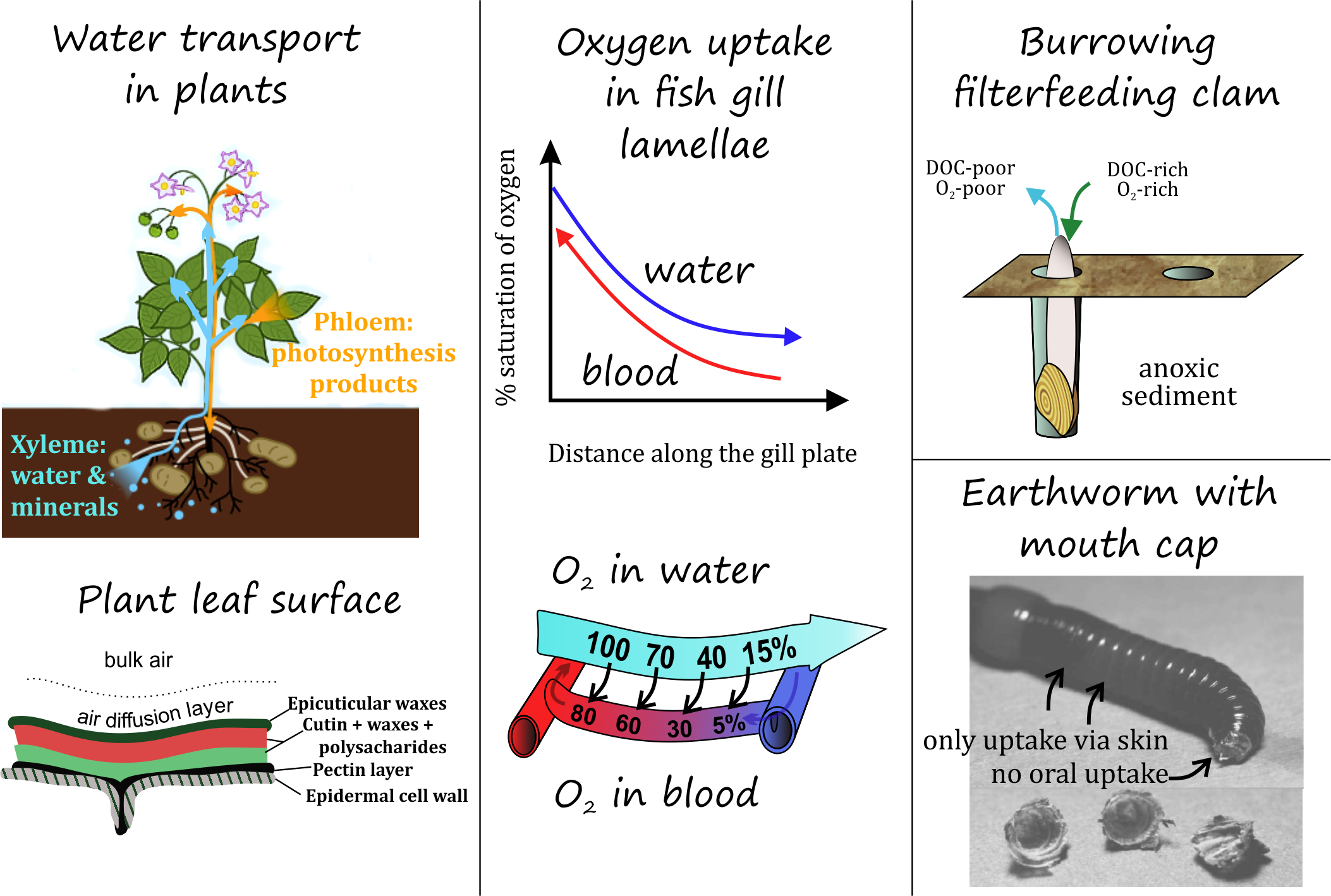
Nearly all plants have roots below ground, a sturdy structure of stem and branches above ground, and leaves. Along with soil pore water, soluble chemicals are readily transported from roots of the plant in the internal circulation stream through xylem cells, which are lined with water impenetrable lignin (see Figure 2). Moderately hydrophobic chemicals (Kow of 1-1000) are rapidly transported from roots to shoots to leaves, while hydrophobic chemicals may be strongly retained on the membranes and cell walls and mostly accumulate in root sections, limiting transport to above-ground plant tissues. Roots may also actively release considerable quantities of chemicals to influence the immediate surrounding media of the roots (rhizosphere), e.g. to stimulate microbial processes or pH in order to release nutrients. These plant root 'exudates' can be ions, small acids, amino acids, sterols, etc. Chemicals that enter plants via leaves, such as pesticides or semi-volatile organic pollutants, can be redistributed to other plant parts via the phloem streams.
The transport through xylem up to higher plant tissues occurs via capillary forces and is enhanced by three passive phenomena:
- the high sugar content in the phloem causing osmotic pressure to attract water from other parts.
- the evaporation of water creates surface tension on thousands of cells that pulls water from the soil through the xylem system.
- the osmotic pressure of root cells compared to soil pore water. Root pressure is highest in the morning before the stomata open and allow transpiration to begin.
As a result of the capillary forces needed to pull water up against gravity, and a certain maximum diameter of the vessels to do so, there is a maximum possible plant height of 122-130 m (Koch et al., 2004) which compares to Redwood trees (Sequoias) reaching a maximum height of 113 m.
Most leaves are covered with a waxy layer, to prevent damage and water evaporation. This wax layer may be 0.3-4.6 µm thick (Moeckel et al., 2008). Large forests provide enormous hydrophobic surfaces to which semi-volatile organic chemicals (SVOC) can bind out of air, which influences the global distribution of chemicals such as PCBs. Partitioning of SVOCs on the vegetation of extended grasslands contaminates the base of the food chain, as well as agricultural and cattle sectors used by humans. The grass/corn-cattle-milk/beef food chain accounts for the largest portion of background exposure of the European and North American population to many persistent SVOCs. The absorption rate of chemicals on the leaves often also depends on the air boundary layer surrounding leaves, which limits diffusion into the leave surfaces. Of course, all kinds of other factors such as wind speed, canopy formation and cuticle thickness also control exchange between leaves and gas phase (see also section 3.1.2 on the Atmosphere). Tiny openings or pores on the lower side of the leaves, called stomata, allow furthermore for gas exchange. In warm conditions, stomata can close to prevent water evaporation, but gas exchange is needed in many plant types to allow for CO2 to be metabolized and the release of O2 that is produced. The waxy layer on leaves can trap gaseous organic chemicals. Many plants, like coniferous trees, produce resins to provide effective defense against insects and diseases, and these resins release large amounts and structurally highly diverse organic volatiles such as terpenes and isoprenes (Michelozzi, 1999). These plant-produced volatiles can even contribute to ozone formation. Plants thus accumulate chemicals from their environment, but also release chemicals into the environment. It thus also matters for the exposure of grazing organisms to certain types of pollutants whether they eat roots, shoots, leaves, seeds or fruits of plants living in contaminated environments.
Organisms using dissolved oxygen
The 'gill' movements of water breathers create a constant flux of chemicals dissolved in bulk water along outer cell membranes (or mucus layers surrounding cell membranes) of gills. A 1 kg rainbow trout fish ventilates about 160 mL/min, so 230 L/day (Consoer et al., 2014). The total gill surface area in a fish depends on species behaviour and weight (active large fish require a lot of oxygen), and equals to about 1-6 cm2 per g fish (Palzenberger & Pohla, 1992). For a 1 kg fish of ~20 cm length, the ~1000 cm2 gill area compares to a ~500 cm2 outer body surface. This results in an effective partitioning of chemicals between water and cell membranes. Within the gills, the cells are in close contact with the blood system of the organism, and the build-up of chemical concentrations in the outer cells provides an effective exchange with the blood stream (or other internal fluids, Figure 2) flushing along that redistribute chemicals to the inner organs. The reverse equally occurs: chemicals dissolved in blood stream coming from organs will also rapidly exchange with bulk external water if concentrations are lower.
Of course, many pollutants can also enter water breathing organisms via food, but the gills-water exchange is very effective in controlling the distribution of chemicals. The salinity of water plays a strong role in the need of water breathing organisms to "drink" water, and hence take in contaminants via this route.
|
BOX 1. Osmoregulation (MSc level) Most aquatic vertebrate animals are osmoregulators: their cells contain a concentration of solutes that is different than the water around them. Fish living in freshwater typically have a cellular osmotic level (300 millOsmoles per Liter, mOsm/L) that is higher than the bulk fresh water (~20-40 mOsm/L), so a lot of water flows passively via the gills (not via the skin) into the tissue of fish. They are thus constantly taking in water (water molecules only) via the gills, which needs to be controlled, e.g. by strongly diluting the urine. They do also take in some water in their gastro-intestinal tract (GIT). Marine fish have similar cellular osmotic levels as freshwater fish, but the salty water (1000 mOsm/L) causes water to move out of the gill tissue through the linings of the fish's gills by osmosis, which needs to be replenished by active intake of salty water, and separate excretion of the salts. Most invertebrate organisms in oceans have an internal overall concentration of dissolved compounds comparable to the water they live in, so that they don't suffer from strong osmotic pressures on their soft tissue (osmoconformers). |
A single adult oyster can cleanse about 200 liters of water per day (https://www.cbf.org/about-the-bay/mo...act-sheet.html). Plans to re-populate the harbour of New York with 1 billion oysters on artificial substrates can have enormous impacts on chemical redistribution. A single 2 cm zebra mussel (Dreissena polymorpha) that inhabits the shallow Lake IJsselmeer (6.05x10¹² L) in can filter about 1 L per day, and the high densities of these and related species in this fresh water lake can turn over the lake volume once or twice per month (Reeders et al., 1989).
Even many soil organism are constantly in contact with wet soil surfaces, and contact between soil pore water and the outer surfaces (gills/soft skin areas) dominates the routes of chemical exchange for many chemicals. Earthworms, for example, do not have lungs and they exchange oxygen through their skin. Earthworms eat bacteria and fungi that grow on dead and decomposing organic matter, and thus act as major organic matter decomposers and recycling of nutrients. Earthworms dramatically alter soil structure, water movement, nutrient dynamics, and plant growth. It is estimated that earthworms turn over the top 15 cm of soil in ten to twenty years (LINK), and so they also are able to mix surface bound pollution into a substantial soil layer. In terms of biomass, earthworms dominate the world of soil invertebrates, including arthropods. In order to better understand how much contamination earthworms take in via food or via their skin, several studies have used earthworms in exposure tests with part of the organisms having their mouth parts sealed with surgical glue (Vijver et al., 2003). Uptake rates of the metals Cd, Cu and Pb in sealed and unsealed earthworms exposed to two contaminated field soils were similar (Vijver et al., 2003), indicating main uptake through the skin of the worms. The uptake rates as well as the maximum accumulation level for several organic contaminants from artificially contaminated soil were also comparable between sealed and non-sealed worms (Jager et al., 2003). The dermal route is thus a highly important uptake route for organic chemicals too. Dermal uptake by soil organisms is generally from the pool of chemicals in the soil pore water, hence the distribution of chemicals between solid particles and organic materials in the soil and the soil pore water is extremely important in driving the dermal uptake of chemicals by earthworms (See section 3.4 on Partitioning and partitioning constants, section 3.5 on Metal speciation and 3.6 on Availability and bioavailability).
Air breathing organisms
Air breathing organisms typically take in less/non-volatile chemicals via food and require active excretion and metabolism for the elimination of these chemicals via e.g. feces and urine. Dermal uptake is generally assumed to be negligible, while the intake of chemicals via air particles can be relatively high, for example of pollutants present in house dust, or contaminants on aerosols. The excretion via air particles is clearly not a dominant route. The chemicals in the food matrix inside the gastro-intestinal tract often first need to be fully dissolved in gut fluids, before they can pass the mucus layers and membranes lining the gastrointestinal tract and enter blood streams for redistribution. However, 'endocytosis' may also result in the uptake of (small) particulate chemicals in cells by first completely surrounding the particle by the membrane, after which the encapsulating membrane buds buds off inside the cell and forms a vesicle. Notwithstanding this endocytosis, chemical fractions of pollutants strongly sorbed to non-digestible parts may not always automatically be taken up from food. Grazing animals typically require microbial conversion in their gut to digest plant material like cellulose and lignin into chemical components that can be taken up as energy source.
Many aquatic foodwebs are structured such that they begin with aquatic plants being eaten by water breathing organisms, with air breathing marine animals or birds on top of the food chain. These air breathing top predators take in pollutants largely through their diet, but lack the effective blood-membrane-water exchange through gills. The blood-membrane-air partitioning in lungs is far less effective in removing chemicals via passive partitioning. For this reason, many top predators of foodwebs have the highest concentrations of pollutants. The chemical distribution in foodwebs will be discussed in more detail in section 4.1.6.
References
Palzenberger & Pohla 1992, Reviews in Fish Biology and Fisheries, 2, 187-216.
Jager, T.; Fleuren, R.H.L.J.; Hogendoorn, E.A.; de Korte, G. 2003. Elucidating the routes of exposure for organic chemicals in the earthworm, Eisenia andrei (Oligochaeta). Environ. Sci. Technol. 37 (15), 3399-3404
Koch et al. 2004, Nature (428) 851-854.
Moeckel et al. 2008, Environ. Sci. Technol. 42, 100-105.
Michelozzi 1999, Defensive roles of terpenoid mixtures in conifers, Acta Botanica Gallica 146 (1), 73-84.
Consoer et al. 2014, Aquatic Toxicology 156, 65-73.
Reeders et al. 1989, Freshwater Biology 22 (1), 133-141.
Vijver et al. 2003, Soil Biology and Biochemistry 35, 125-132.
Goss et al. 2018, Chemosphere 199, 174-181.
Explain whether a lean fish of 1 kg likely contains a lower concentration of hydrophobic pollutant as a 1 kg fatty fish caught in the same lake.
Explain how bivalves (clams, muscles, oysters) can reduce contamination with a hydrophobic chemical from a lake
In many countries, the levels of water pollution have been strongly reduced compared to 30 years ago, but a lot of sediments are still contaminated with historic pollutants that strongly bind to the sediment particles. Explain how historic contamination in a sediment can be brought into suspension by benthic organisms.
Discuss whether the internal concentrations of very hydrophobic chemicals in fatty fish gets higher or lower during an extended period of starvation, e.g. during migration towards breeding grounds. Note that very hydrophobic chemicals may have elimination half lives of months or even longer.
Discuss whether the internal concentrations of very hydrophobic chemicals in female organisms gets higher or lower during a reproduction cycle, e.g. by generating offspring and or lactation. Note that very hydrophobic chemicals may have elimination half lives of months or even longer.