18.1: Helix–Coil Transition

Cooperativity plays an important role in the description of the helix–coil transition, which refers to the reversible transition of macromolecules between coil and extended helical structures. This phenomenon was observed by Paul Doty in the 1950s for the conversion of polypeptides between a coil and α-helical form,² and for the melting and hybridization of DNA.³ Bruno Zimm developed a statistical theory with J. Bragg that described the helix–coil transition, which forms the basis of our discussion.⁴

One of the observations that motivated this work is shown in the figure below. The fraction of helical structure observed in the polypeptide poly-benzylglutamate showed a temperature-dependent melting behavior in which the steepness of the transition increased with polymer chain length. This length dependence indicates a higher probability of forming helices when more residues are present, and that the linkages do not act independently. This suggests a two-step mechanism. The rate-limiting step of forming an \(α\) helix is the nucleation of a single hydrogen bonded residue \(i → i+4\) loop. Once this occurs, the addition of further hydrogen bonds to extend this helix is much easier and occurs in rapid succession.

To model this behavior, we imagine that the polypeptide consists of a chain of segments that can take on two configurations, H or C.

H: helix (decreases entropy but also lower enthalpy)

C: coil (raises entropy)

To specify the state of a conformation through a sequence, i.e.,

...HCHHHHCCCCHHH...

Remember to not take this too literally, and be flexible in the interpretation of your model. Although this model was derived with an \(α\)-helix formation in polypeptides in mind, in a more general sense \(H\) and \(C\) do not necessarily refer explicitly to residues of a sequence, but just for independently interacting regions.

If there are \(n\) segments, these can be divided into \(n_H\) helical and \(n_C\) coil segments.

\[n_H + n_C = n \nonumber \]

The segments need not correspond directly to amino acids, but structurally and energetically distinct regions. Our goal will be to calculate the fractional helicity of this system \(\theta_H\) as a function of temperature, by calculating the conformational partition function, q_conf, by an explicit summation over i microstates, Boltzmann weighed by the microstate energy E_i:

\[ q_{\mathrm{conf}} (n) = \sum_{i\, \mathrm{config.}} e^{-E_i/k_BT} \]

Non‐cooperative Model

We start our analysis by discussing a non-cooperative model. We assume:

• Each segment can switch conformation between H and C independently of the others.
• The formation of H from C lowers the configurational energy by \(\Delta \epsilon .\, \Delta \epsilon = E_H - E_C\) is a free-energy change per residue, where \(\Delta \epsilon < 0\). We will take the coil state to be the reference energy E_C = 0.
• Therefore the energy of the system is determined from the number of H residues present, not the specific sequence of H and C segments.

\[ E_i = E(n_H) = n_H\Delta \epsilon \nonumber \]

Then, we can calculate q_conf using g(n,n_H), the degeneracy of distinguishable states for a polymer of length n with n_H helical segments. The conformational partition function is obtained by

\[q_{\mathrm{conf}}(n) = \sum_{n_H=0}^n g(n,n_H) e^{-n_H \Delta \epsilon / k_BT} \]

In evaluating the partition functions in helix–coil transition models, it is particularly useful to define a “statistical weight” for the helical configuration. It describes the influence of having an H on the probability of observing a particular configuration at kBT:

\[s = e^{-\Delta \epsilon / k_BT} \]

For the present model, we can think of s as an equilibrium constant for the process of adding a helical residue to a sequence:

\[s = \dfrac{P(n_H+1)}{P(n_H)} \nonumber \]

This equilibrium constant is related to the free energy change for adding a helical residue to the growing chain. Then we can write eq. (18.1.2) as

\[q_{\mathrm{conf}}(n) = \sum_{n_H=0}^n g(n,n_H) s^{n_H} \nonumber \]

Since there are only two possible configurations (H and C), the degeneracy of configurations with \(n_H\) helical segments in a chain of length n is given by the binomial coefficients:

\[ g(n,n_H) = \dfrac{n!}{n_H!n_C!} = \begin{pmatrix} n \\ n_H \end{pmatrix} \]

since \(n_C=n-n_H\). Then using the binomial theorem, we obtain

\[q_{\mathrm{conf}}(n) = (1+s)^n \]

Also, the probability of a chain with n segments having n_H helical linkages is

\[P(n,n_H) = \dfrac{g(n,n_H)e^{-E(n_H)/k_BT}}{q_{\mathrm{conf}}} = \begin{pmatrix} n \\ n_H \end{pmatrix} \dfrac{s^{n_H}}{(1+s)^n} \]

Example: n = 4

The conformations available are at right. The molecular conformational partition function is

\(\begin{aligned} q_{\mathrm{conf}} &= 1+4e^{-\Delta \epsilon /k_BT} +6e^{-2\Delta \epsilon /k_BT} +4e^{-3\Delta \epsilon /k_BT} +e^{-4\Delta \epsilon /k_BT} \\ &= 1+4s+6s^2+4s^3+s^4 \\ &= (1+s)^4 \end{aligned} \)

The last step follows from Pascal’s Rule for binomial coefficients. From eq. (18.1.6), the probability of having two helical residues in a four-residue sequence is:

\[P(4,2) = \dfrac{6s^2}{(1+s)^4} \nonumber \]

To relate this to an observable quantity, we define the fractional helicity, the average fraction of residues that are in the H form.

\[ \theta_H = \dfrac{\langle n_H \rangle}{n} \]

\[ \langle n_H \rangle = \sum_{n_H = 0}^{n} n_HP(n,n_H) \]

Using this amazing little identity, which we derive below,

\[ \langle n_H \rangle = \dfrac{s}{q} \dfrac{\partial q}{\partial s} \]

You can use eq. (18.1.5) to show:

\[ \langle n_H \rangle = \dfrac{ns}{1+s} \]

and

\[ \theta_H = \dfrac{s}{1+s} \]

This takes the same form as one would expect for the simple chemical equilibrium of an \(C \rightleftharpoons H\) molecular reaction. If we define the equilibrium constant K_HC = [H]/[C], then the fraction of molecules in the H state is \(\theta_H = [H]/([C]+[H]) = K_{HC}/(1+K_{HC})\). In this limit s = K_HC.

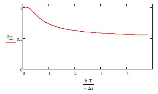
Below we plot eq. (18.1.11), choosing Δε to be independent of temperature. θ_H is a smooth and slowly varying function of T and does not show cooperative behavior. Its high temperature limit is θ_H= 0.5, reflecting the fact that in the absence of barriers, the H and C configurations are equally probable for every residue.

We can look a bit deeper at what is happening with the structures present by plotting the probability distribution function for finding nH helical segments within a chain of length n, eq. (18.1.6), and the associated energy landscape (a potential of mean force):

\[F(n,n_H) = -Nk_BT\ln{[P(n,n_H)]} \approx -Nk_BT \ln{[g(n,n_H)s^{n_H}]} \nonumber \]

The maximum probability and free-energy minimum is located at full helix content at the lowest temperature, and gradually shifts toward nH/n = 0.5 with increasing temperature. The probability density appears Gaussian, and the corresponding free energy appears parabolic. Using similar methods to that described above, we can show that the variance in this distribution scales as n−1/2.The presence of a single shifting minimum is referred to as a transition in a one-state system, rather than two-state behavior expected for phase transitions. Here nH is the order parameter that characterizes the extend of folding of the helix.

Where does eq. (18.1.9) come from? For the moment, we will drop the “conf” and “H” subscripts, mainly to write things more compactly, but also to emphasize the generality of this method to all polynomial expansions. Using eq. (18.1.2), \(q= \sum_n gs^n \), and recognizing that g is not a function of s: \[ \begin{aligned} \dfrac{\partial q}{\partial s} &= \sum_n ngs^{n-1} \\ &= \dfrac{1}{s}\sum_nngs^n \end{aligned} \] \[\] From eq. (18.1.6), \(P_n = gs^n/1 \), we can write this in terms of the helical segment probability \[ \dfrac{1}{q} \dfrac{\partial q}{\partial s} = \dfrac{1}{s}\sum_nnP_n \] Comparing eq. (18.1.13) with eq. (18.1.12), \( \boldsymbol{\langle} n \boldsymbol{\rangle} = \sum_nnP_n \), we see that \[\dfrac{s}{q} \dfrac{\partial q}{\partial s} = \langle n \rangle \quad \mathrm{or} \quad \dfrac{\partial \ln{q}}{\partial \ln{s}} = \boldsymbol{\langle} n \boldsymbol{\rangle} \] This method of obtaining averages from derivatives of a polynomial appears regularly in statistical mechanics.^5

Cooperative Zimm–Bragg Model

Let’s modify the model to add an element of cooperativity to the segments in the chain. In order to form a helix, you need to nucleate a helical turn and then adding adjacent helical segments is easier. The probability of forming a turn is relatively low, meaning the free energy barrier for nucleation of one H in a sequence of C is relatively high: \(\Delta G_{nuc}>0\). However the free-energy change per residue for forming H from C within a helical stretch, \(\Delta G_{HC} \), stabilizes the growing helix. Based on these free energies, we define statistical weights:

\[ s = e^{-\Delta G_{HC}/k_BT} \nonumber \]

\[\sigma = e^{-\Delta{nuc}/k_BT}\nonumber \]

s and σ are also known as the Zimm–Bragg parameters. Here, s is the statistical weight to add one helical segment to an existing continuous sequence (or stretch) of H, which we interpret as an equilibrium constant:

\[ s = \dfrac{[...CHHHHCC...]}{[...CHHHCCC...]}= \dfrac{P_H(n_H+1)}{P_H(n_H)} \nonumber \]

σ is the statistical weight for each stretch of H. This is purely to reflect the probability of forming a new helical segment within a stretch of C. The energy benefit of making the helical form is additional:

\[ \sigma s = \dfrac{[...CCCHCC...]}{[...CCCCCC...]}= \dfrac{P_H(\nu_H+1)}{P_H(\nu_H)} \nonumber \]

\(\nu \) is the number of helical stretch segments in a chain. Note that the formation of the first helical segment has a contribution from both the nucleation barrier (σ) and the formation of the first stabilizing interaction (s). The statistical weight for a particular microstate is then \(e^{-E_i/k_BT } = s^{n_H}\sigma^{\nu_H}\) Since \(\Delta G_{nucl} will be large and positive, σ≪ 1. Also, we take s > 1, and the presence of cooperativity will mainly hinge on σ ≪ s.

Example

A 35 segment chain has 235 = 3.4×1010 possible configurations. This particular microstate has fifteen helical segments (nH = 16) partitioned into three helical stretches (νH = 3):

\[ CCCCCC \underbrace{HHHHH}_5 CCC \underbrace{H}_1 CCCCCCCC \underbrace{HHHHHHHHHH}_{10}CC \nonumber \]

We ignore all Cs since the C state is the ground state and their statistical weight is 1.

\[ e^{-E_i/k_BT} = s^{n_H}\sigma^{\nu_H} = s^{16}\sigma^3 \nonumber \]

Now the partition function involves a sum over all possible helical segments and stretches:

\[q_{conf}(n) = \sum_{n_H=0}^n \sum_{\nu_H = 0}^{\nu_{max}} g(n,n_H,\nu_H )s^{n_H}\sigma^{\nu_H} \]

Since the all-coil state (n_H= 0) is the reference state, it contributes a value of 1 to the partition function (the leading term in the summation). Therefore, the probability of observing the all-coil state is

\[P(n,n_H = 0) = q_{conf}^{-1} \]

From eq. (18.1.15), the mean number of helical residues is

\[ \langle n_H \rangle =\dfrac{1}{q_{conf}} \sum_{n_H=0}^n \sum_{\nu_H = 0}^{\nu_{max}} n_H g(n,n_H,\nu_H) s^{n_H}\sigma^{\nu_H} \nonumber \]

In these equations, ν_max refers to the maximum number of helical stretches for a given n_H, n_H/2 for even n_H and (n_H/2)+1 for odd n_H.

Zipper model

As a next step, we examine what happens with the simplifying assumption that one helical stretch is allowed. This is the single stretch approximation or the zipper model, in which conversion to a helix proceeds quickly once a single turn has been nucleated. This is reasonable for short chains in which two stretches are unlikely due to steric constraints. For the single stretch case, we only need to account for ν_H= 0 and 1. For ν_H = 0 the system is all coil (n_H = 0) and there is only one microstate to count, g(n,0,0) = 1. For a single helical stretch we need to accounts for the number of ways of positioning a single helical stretch of n_H residues on a chain of length n: g(n,n_H,1) = n-n_H+1. Then the partition function, eq. (18.1.15), is

\[q_{zip}(n) = 1+\sigma \sum_{n_H=1}^n (n-n_H+1)s^{n_H} \]

We can evaluate these sums using the relations

\[ \begin{aligned} \sum_{n_H=1}^n &= \dfrac{s^{n+1}-s}{s-1} \\ \sum_{n_H=1}^n n_H s^{n_H} &= \dfrac{s}{(s-1)^2} \left[ ns^{n+1}-(n+1)s^n +1 \right] \end{aligned} \]

which leads to

\[ q_{zip}(n) = 1+ \dfrac{\sigma s^2}{(s-1)^2} \left( s^n + \dfrac{n}{s}-(n+1) \right) \nonumber \]

Following the general expression in eq. (18.1.6), and counting the degeneracy of ways to place a stretch of n_H segments, the probability distribution of helical segments is

\[ P_H(n,n_H) = \dfrac{(n-n_H+1)\sigma s^{n_H}}{q_{conf}} \qquad \qquad 1\leq n_H \leq n\]

This expression does not apply to the case n_H = 0, for which we turn to eq. (18.1.16). The helical fraction is obtained from \( \theta_H = \frac{s}{n}(\partial \ln {q_{zip}}/\partial s) \) :

\[ \theta_H = \dfrac{\sigma s}{(s-1)^3} \left( \dfrac{ns^{n+2}-(n+2)s^{n+1}+(n+2)s - n}{n \{ 1+\left( \sigma s/(s-1)^2 \right) \left( s^{n+1} + n - (n+1)s \right) \}} \right) \nonumber \]

Multiple stretches

Expressions for the full partition function of chains with length n, eq. (18.1.15), can be evaluated for one-dimensional models that account for nearest neighbor interactions (Ising model) using an approach based on a statistical weight matrix, M. You can show that the Zimm–Bragg partition function can be written as a product of matrices of the form

\[ \begin{aligned} q_{conf} (n) &= \begin{pmatrix} 1 &0 \end{pmatrix} \bf{M}^n \begin{pmatrix} 1 \\ 1 \end{pmatrix} \\ \bf{M} &= \begin{pmatrix} 1&\sigma s \\ 1&s \end{pmatrix} \end{aligned} \]

Each matrix represents possible configurations of two adjoining partners, and M raised to the nth power gives all configurations for a chain of length n. This form also indicates that we can obtain a closed form for q_conf from the eigenvalues of M raised to the n^th power. If T is the transformation that diagonalizes M, Λ = T^‒1MT, then Mⁿ = TΛⁿT^‒1. This approach allows us to write

\[ q_{conf} = \underset{ \sim }{\lambda}^{-1} \left( \lambda^{n+1}_+ (1-\lambda_-)-\lambda^{n+1}_-(1-\lambda_+)\right) \nonumber \]

\(\mathrm{with} \begin{aligned} \qquad \qquad \qquad \qquad \qquad \qquad \qquad \qquad \qquad \qquad \qquad \qquad &\lambda_{\pm} = \frac{1}{2} \left( (1-s) \pm \underset{ \sim }{\lambda} \right) \\ &\underset{ \sim }{\lambda} = \lambda_+ - \lambda_- = \left( (1-s)^2+4\sigma s\right)^{-1/2} \end{aligned} \)

and the fractional helicity is obtained from

\[\theta_H = \dfrac{\langle n_H \rangle}{n}= \dfrac{s}{n} \dfrac{\partial \ln{q_{conf}}}{\partial s} \]

Simplifying these expressions for the limit of long chains \( (n \rightarrow \infty , \lambda^{n+1}_+ \gg \lambda_-^{n+1} ) \), one finds

\[ q_{conf} \approx \left( \dfrac{1+s+\underset{ \sim }{\lambda}}{2} \right)^n \nonumber \]

and \[ \theta_H = s \left( \dfrac{1+\frac{1}{\underset{ \sim }{\lambda}}(s-1+2\sigma }{1+s+\underset{ \sim }{\lambda}} \right) \]

Note that when you set σ =1, you recover the noncooperative expression, eq. (18.1.11). When s→1, θ_H→0.5.

Below, we examine the transition behavior in the large n limit from eq. (18.1.20) as a function of the cooperativity parameter σ. We note that a sharp transition between an ensemble that is mostly coil to one that is mostly helix occurs near s = 1, the point where these states exist with equal probability. When the \(C\rightleftharpoons H\) equilibrium shifts slightly to favor H (s slightly greater than 1), most of the sample quickly converts to helical form. When the equilibrium shifts slightly toward C, most of the sample follows. As σ decreases, the steepness of this transition grows as \( (d\theta / ds)_{s=1}=1/4\sigma^{1/2}\). Therefore, we conclude that highly cooperative transitions will have s ≈ 1 and σ≪ s. In practice for polypeptides, we find that σ/s lies between 5×10^–3 and 5×10^–5.

Next, we explore the chain-length dependence for finite chains. We find that the cooperativity of this transition, observed through the steepness of the curve at θ_H = 0.5 increases with n. We also observe that the observed midpoint (θ_H = 0.5) lies at s > 1, where the single linkage equilibrium favors the H form. This reflects the constraints on the length of helical stretches available a given chain.

Temperature Dependence

Now let’s describe the temperature dependence of the cooperative model. The helix–coil transition shows a cooperative melting transition, where heating the sample a few degrees causes a dramatic change from a sample that is primarily in the C form to one that is primarily H. Multiple temperature-dependent factors make this a bit difficult to deal with analytically, therefore we focus on the behavior at the melting temperature T_m, which we define as the point where θ_H(T_M) = 0.5.

Look at the slope of θ at T_m. From chain rule:

\[ \dfrac{d\theta }{dT} = \dfrac{d\theta}{ds} \cdot \dfrac{ds}{dT} = \dfrac{d\theta}{ds} \cdot s\dfrac{d\ln{s}}{dT} \nonumber \]

Since we interpret s as an equilibrium constant for the addition of one helical residue to a stretch, we can write a van’t Hoff relation

\[ \dfrac{d\ln{s}}{dT} = \dfrac{\Delta H^0_{HC}}{k_BT^2} \nonumber \]

Note that this relation assumes that ΔH⁰ is independent of temperature, which generally is a concern, but we will not worry too much since we are just evaluating this at T_M. Next we focus our discussion on the high n limit. From the Zimm–Bragg model:

\[ \left( \dfrac{d\theta}{ds} \right)_{s=1} = \dfrac{1}{4\sigma^{1/2}} \nonumber \]

Then, we set s(T_m) = 1, and combine these results to give the slope of the melting curve at T_m:

\[ \left( \dfrac{d\theta }{dT} \right)_{T=T_m} = \dfrac{\Delta H^0_{HC}}{4\sigma^{1/2}k_BT^2_m} \nonumber \]

The slope of \(\theta \mathrm{at} T_m\) has units of inverse temperature, so we can also express this as a transition width: \(\Delta T_m = (d\theta / dT)^{-1}_{T_m}\).

Keep in mind this van’t Hoff analysis comes with some real limitations when applied to experimental data. It does not account for the finite size of the system, which we have seen shifts s(T_m) to be >1, and the knowledge of parameters at T_m does not necessarily translate to other temperatures. To the extent that you can apply the assumptions, the van’t Hoff expression can also be used to predict the helical fraction as a function of temperature in the vicinity of T_M using

\(\ln{s} = \dfrac{\Delta H^0_{HC}}{k_B}\left( \dfrac{1}{T_M}-\dfrac{1}{T} \right) \)

and assuming that σ is independent of temperature.

Below we show the length dependence of the melting temperature. As the length of the chain approaches infinite, the helix/coil transition becomes a step function in temperature. This trend matches the expectations for a phase transition: in the thermodynamic limit, the infinite system, will show discontinuous behavior. For finite lengths, the melting temperature Tm is lower that for the infinite chain (T_m,∞), but approaches this value for n>300.

Calorimetric parameters for polypeptide chains

Side-chain only has a small effect on the helix–coil propagation parameter:

	Sample	\(\Delta H_{HC}^0\) (kcal mol^-1 residue^-1)	\(\sigma\)	Other
	Alanine-rich peptides Ac-Y(AEAAKA)8F-NH2 Ac-(AAKAA)kY-NH2	-0.95 to -1.3	0.002
	Poly(L-lysine) Poly(L-glutamate)	-1.1	0.0025
	Poly-alanine	-0.95	0.003	s(0°C)=1.35;
	Alanine oligomers	-0.85		ΔS^0=3 cal mol^-1 res^-1 K^-1
	Various homopolypeptides	~4 kJ		ΔCP=-32 J/mol K res^-1

Free‐Energy Landscape

Finally, we investigate the free-energy landscape for the Zimm–Bragg model of the helix–coil transition. The figure below shows the helical probability distribution and corresponding energy landscape for different values of the reduced temperature kBT/Δε for a chain length of n=40 and σ=10-3. Note that P(nH) is calculated from eq. (18.1.18) for all but the all-coil state, which comes from eq. (18.1.16).

The cooperative model shows two-state behavior. At low temperature and high temperature, the system is almost entirely in the all-helix or all-coil configuration, respectively; however, at intermediate temperatures, the distribution of helical configurations can be very broad. The least probable configuration is a chain with only one helical segment.

This behavior looks much closer to the two-state behavior expected from phase-transition behavior. The free energy has minima for n_H= 0 and for n_H> 1, and the free energy difference between these states shifts with temperature to favor one or the other minimum.

___________________________________________________________________

1. C. R. Cantor and P. R. Schimmel, Biophysical Chemistry Part III: The Behavior of Biological Macromolecules. (W. H. Freeman, San Francisco, 1980), Ch. 20; D. Poland and H. A. Scheraga, Theory of Helix–Coil Transitions in Biopolymers. (Academic Press, New York, 1970).

2. P. Doty, A. M. Holtzer, J. H. Bradbury and E. R. Blout, POLYPEPTIDES. II. THE CONFIGURATION OF POLYMERS OF γ-BENZYL-L-GLUTAMATE IN Solution, J. Am. Chem. Soc.76 (17), 4493-4494 (1954); P. Doty and J. T. Yang, POLYPEPTIDES. VII. POLY-γ-BENZYL-L-GLUTAMATE: THE HELIX-COIL TRANSITION IN Solution, J. Am. Chem. Soc. 78 (2), 498-500 (1956).

3. J. Marmur and P. Doty, Heterogeneity in Deoxyribonucleic Acids: I. Dependence on Composition of the Configurational Stability of Deoxyribonucleic Acids, Nature 183 (4673), 1427-1429 (1959).

4. B. H. Zimm and J. K. Bragg, Theory of the phase transition between helix and random coil in polypeptide chains, J. Chem. Phys. 31, 526-535 (1959).

5. K. Dill and S. Bromberg, Molecular Driving Forces: Statistical Thermodynamics in Biology, Chemistry, Physics, and Nanoscience. (Taylor & Francis Group, New York, 2010), Appendix C p. 705.