5.2: Hydrophobic Solvation- Solute Size Effect

To create a new interface there are enthalpic and entropic penalties. The influence of each of these factors depends on the size of the solute (R) relative to the scale of hydrogen bonding structure in the liquid (correlation length, \(\ell\), ~0.5–1.0 nm).

For small solutes (\(R < \ell\) ): Network deformation

The solute can insert itself into the hydrogen bond network without breaking hydrogen bonds. It may strain the HBs (\(\Delta H > 0\)) and reduce the configurational entropy (\(\Delta S < 0\)), but the liquid mostly maintains hydrogen bonds intact. We expect the free energy of this process to scale as volume of the solute \(\Delta G_{\text{sol}} (R < \ell) \propto R^3\).

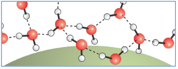
For large solutes, \(R > \ell\): Creating an interface

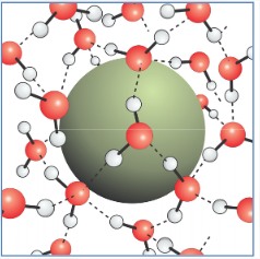
The hydrogen bond network can no longer maintain all of its HBs between water molecules. The low energy state involves dangling hydrogen bonds at the surface. One in three surface water molecules has a dangling hydrogen bond, i.e., on average five of six hydrogen bonds of the bulk are maintained at the interface.

We expect \(\Delta G_{\text{sol}}\) to scale as the surface area \(\Delta G_{\text{sol}} (R > \ell) \propto R^2\). Of course, large solutes also have a large volume displacement term. Since the system will always seek to minimize the free energy, there will be a point at which the \(R^3\) term grows faster with solute radius than the \(R^2\) term, so large solutes are dominated by the surface term.

Calculating \(\Delta G\) for Forming a Cavity in Water

Let’s investigate the energy required to form cavities in water using a purely thermodynamic approach. To put a large cavity (\(R > \ell\)) into water, we are creating a new liquid–vapor interface for the cavity. So we can calculate the energy to create a cavity using the surface tension of water. Thermodynamically, the surface tension \(\gamma\) is the energy required to deform a liquid–vapor interface: \(\gamma=(\partial U / \partial a)_{N, V, T}\), where \(a\) is the surface area. So we can write the change in energy as a result of inserting a spherical cavity into water as the product of the surface tension of water times the surface area of the cavity,

\[U(R)=4 \pi R^{2} \gamma \nonumber\]

In principle, the experimentally determined \(\gamma\) should include entropic and enthalpic contributions to altering the hydrogen bond network at a surface, so we associate this with \(\Delta G_{\text{sol}}\). For water at \(300\ K\), \(\gamma = 72\ pN/nm\). \(\gamma\) varies from \(75\ pN/nm\) at \(0\ ^{\circ}C\) to \(60\ pN/nm\) at \(100\ ^{\circ}C\).

The surface tension can also be considered a surface energy per unit area: which can also be considered a surface energy, i.e., \(\gamma = 72\ mJ/m^2\). To relate this to a molecular scale quantity, we can estimate the surface area per water molecule in a spherical cavity. The molecular volume of bulk water deduced from its density is \(3.0 \times 10^{-26}\ \text{L/molecule}\), and the corresponding surface area per molecule deduced from geometric arguments is \(\sim 10 \mathring{A}^2\). This area allows us to express \(\gamma \approx 4.3\ kJ/mol\), which is on the order of the strength of hydrogen bonds in water.

For small cavities (\(R < \ell\)), the considerations are different since we are not breaking hydrogen bonds. Here we are just constraining the configurational space of the cavity and interface, which should scale as volume. We define

\[\Delta G_{\text{sol}}(R < \ell) = \dfrac{4 \pi R^{3}}{3} \rho_{E} \nonumber\]

where \(\rho_E\) is an energy density¹.

\[\rho_{E} \approx 240 \times 10^{-9} \ pJ/nm^{3} = 240 \ pN/nm^{-2}\nonumber\]

Remembering that \(-\partial G /\left.\partial V\right|_{N, T}=p\), the energy density corresponds to units of pressure with a value \(\rho_E = 2.4 \times 10^3\) atm. If we divide \(\rho_E\) by the molarity of water (55M), then we find it can be expressed as \(4.4\ kJ/mol\), similar to the surface free energy value deduced.

So combining the surface and volume terms we write

\[\Delta G_{\text{sol}}(R)=4 \pi \gamma R^{2}+\dfrac{4}{3} \pi R^{3} \rho_{E}\nonumber\]

Alternatively, we can define an effective length scale (radius) for the scaling of this interaction

\[\dfrac{\Delta G_{\text{sol}}}{k_{B} T} = \left ( \dfrac{R}{R_{\text{surf}}} \right )^{2} + \left (\dfrac{R}{R_{V}} \right) ^{3} \quad \quad \quad R_{\text{surf}}=\sqrt{\dfrac{k_{B} T}{4 \pi \gamma}} \quad R_{V} = \left (\dfrac{3 k_{B} T}{4 \pi \rho_{E}} \right)^{1/3} \nonumber\]

where \(R_{\text{surf}} = 0.067\ nm\) and \(R_V = 1.6\ nm\) at \(300\ K\). We can assess the crossover from volume-dominated to area-dominated hydrophobic solvation effects by setting these terms equal and finding that this occurs when \(R = 3\gamma /\rho_E = 0.9\ nm\). The figure below illustrates this behavior and compares it with results of MD simulations of a sphere in water.

An alternate approach to describing the molar free energy of solvation for a hydrophobic sphere of radius \(r\) equates it with the probability of finding a cavity of radius \(r\):

\[\Delta G = -k_B T \ln P(r)\nonumber\]

\[\begin{array} {rcl} {P(r)} & = & {\dfrac{e^{-U(r)/k_B T}}{\int_0^{\infty} e^{-U(r)/k_B T} dr} = \dfrac{\exp \left [\dfrac{-4\pi \gamma r^2}{k_B T} \right]}{\dfrac{1}{2} \sqrt{\dfrac{k_B T}{4\gamma}}}} \\ {} & = & {\dfrac{2}{\sqrt{\pi} R_{\text{surf}}} \exp [-r^2/R_{\text{surf}}^2]} \end{array} \nonumber\]

This leads to an expression much like we previously described for large cavities. It is instructive to determine for water @ \(300\ K\):

\[\langle r\rangle=\int_{0}^{\infty} dr\ r\ P(r)=\pi^{-1 / 2} R_{\text{suff}}=\dfrac{1}{2 \pi} \left (\dfrac{k_{B} T}{\gamma} \right)^{1/2}=0.038\ nm \nonumber\]

This is very small, but agrees well with simulations. (There is not much free volume in water!) However, when you repeat this to find the variance in the size of the cavities \(\delta r = (\langle r^2 \rangle - \langle r \rangle^2)^{1/2}\), we find \(\delta r = 0.028\ nm\). So the fluctuations in size are of the same scale as the average and therefore quite large in a relative sense, but still less than the size of a water molecule.

Simulations give the equilibrium distribution of cavities in water

\[\Delta \mu^0 = -k_B T \ln (P) \nonumber\]

_______________________________________

1. D. Chandler, Interfaces and the driving force of hydrophobic assembly, Nature 437, 640–647 (2005).