
Cyclic Voltammetry
- Page ID
- 311
\( \newcommand{\vecs}[1]{\overset { \scriptstyle \rightharpoonup} {\mathbf{#1}} } \)
\( \newcommand{\vecd}[1]{\overset{-\!-\!\rightharpoonup}{\vphantom{a}\smash {#1}}} \)
\( \newcommand{\dsum}{\displaystyle\sum\limits} \)
\( \newcommand{\dint}{\displaystyle\int\limits} \)
\( \newcommand{\dlim}{\displaystyle\lim\limits} \)
\( \newcommand{\id}{\mathrm{id}}\) \( \newcommand{\Span}{\mathrm{span}}\)
( \newcommand{\kernel}{\mathrm{null}\,}\) \( \newcommand{\range}{\mathrm{range}\,}\)
\( \newcommand{\RealPart}{\mathrm{Re}}\) \( \newcommand{\ImaginaryPart}{\mathrm{Im}}\)
\( \newcommand{\Argument}{\mathrm{Arg}}\) \( \newcommand{\norm}[1]{\| #1 \|}\)
\( \newcommand{\inner}[2]{\langle #1, #2 \rangle}\)
\( \newcommand{\Span}{\mathrm{span}}\)
\( \newcommand{\id}{\mathrm{id}}\)
\( \newcommand{\Span}{\mathrm{span}}\)
\( \newcommand{\kernel}{\mathrm{null}\,}\)
\( \newcommand{\range}{\mathrm{range}\,}\)
\( \newcommand{\RealPart}{\mathrm{Re}}\)
\( \newcommand{\ImaginaryPart}{\mathrm{Im}}\)
\( \newcommand{\Argument}{\mathrm{Arg}}\)
\( \newcommand{\norm}[1]{\| #1 \|}\)
\( \newcommand{\inner}[2]{\langle #1, #2 \rangle}\)
\( \newcommand{\Span}{\mathrm{span}}\) \( \newcommand{\AA}{\unicode[.8,0]{x212B}}\)
\( \newcommand{\vectorA}[1]{\vec{#1}} % arrow\)
\( \newcommand{\vectorAt}[1]{\vec{\text{#1}}} % arrow\)
\( \newcommand{\vectorB}[1]{\overset { \scriptstyle \rightharpoonup} {\mathbf{#1}} } \)
\( \newcommand{\vectorC}[1]{\textbf{#1}} \)
\( \newcommand{\vectorD}[1]{\overrightarrow{#1}} \)
\( \newcommand{\vectorDt}[1]{\overrightarrow{\text{#1}}} \)
\( \newcommand{\vectE}[1]{\overset{-\!-\!\rightharpoonup}{\vphantom{a}\smash{\mathbf {#1}}}} \)
\( \newcommand{\vecs}[1]{\overset { \scriptstyle \rightharpoonup} {\mathbf{#1}} } \)
\(\newcommand{\longvect}{\overrightarrow}\)
\( \newcommand{\vecd}[1]{\overset{-\!-\!\rightharpoonup}{\vphantom{a}\smash {#1}}} \)
\(\newcommand{\avec}{\mathbf a}\) \(\newcommand{\bvec}{\mathbf b}\) \(\newcommand{\cvec}{\mathbf c}\) \(\newcommand{\dvec}{\mathbf d}\) \(\newcommand{\dtil}{\widetilde{\mathbf d}}\) \(\newcommand{\evec}{\mathbf e}\) \(\newcommand{\fvec}{\mathbf f}\) \(\newcommand{\nvec}{\mathbf n}\) \(\newcommand{\pvec}{\mathbf p}\) \(\newcommand{\qvec}{\mathbf q}\) \(\newcommand{\svec}{\mathbf s}\) \(\newcommand{\tvec}{\mathbf t}\) \(\newcommand{\uvec}{\mathbf u}\) \(\newcommand{\vvec}{\mathbf v}\) \(\newcommand{\wvec}{\mathbf w}\) \(\newcommand{\xvec}{\mathbf x}\) \(\newcommand{\yvec}{\mathbf y}\) \(\newcommand{\zvec}{\mathbf z}\) \(\newcommand{\rvec}{\mathbf r}\) \(\newcommand{\mvec}{\mathbf m}\) \(\newcommand{\zerovec}{\mathbf 0}\) \(\newcommand{\onevec}{\mathbf 1}\) \(\newcommand{\real}{\mathbb R}\) \(\newcommand{\twovec}[2]{\left[\begin{array}{r}#1 \\ #2 \end{array}\right]}\) \(\newcommand{\ctwovec}[2]{\left[\begin{array}{c}#1 \\ #2 \end{array}\right]}\) \(\newcommand{\threevec}[3]{\left[\begin{array}{r}#1 \\ #2 \\ #3 \end{array}\right]}\) \(\newcommand{\cthreevec}[3]{\left[\begin{array}{c}#1 \\ #2 \\ #3 \end{array}\right]}\) \(\newcommand{\fourvec}[4]{\left[\begin{array}{r}#1 \\ #2 \\ #3 \\ #4 \end{array}\right]}\) \(\newcommand{\cfourvec}[4]{\left[\begin{array}{c}#1 \\ #2 \\ #3 \\ #4 \end{array}\right]}\) \(\newcommand{\fivevec}[5]{\left[\begin{array}{r}#1 \\ #2 \\ #3 \\ #4 \\ #5 \\ \end{array}\right]}\) \(\newcommand{\cfivevec}[5]{\left[\begin{array}{c}#1 \\ #2 \\ #3 \\ #4 \\ #5 \\ \end{array}\right]}\) \(\newcommand{\mattwo}[4]{\left[\begin{array}{rr}#1 \amp #2 \\ #3 \amp #4 \\ \end{array}\right]}\) \(\newcommand{\laspan}[1]{\text{Span}\{#1\}}\) \(\newcommand{\bcal}{\cal B}\) \(\newcommand{\ccal}{\cal C}\) \(\newcommand{\scal}{\cal S}\) \(\newcommand{\wcal}{\cal W}\) \(\newcommand{\ecal}{\cal E}\) \(\newcommand{\coords}[2]{\left\{#1\right\}_{#2}}\) \(\newcommand{\gray}[1]{\color{gray}{#1}}\) \(\newcommand{\lgray}[1]{\color{lightgray}{#1}}\) \(\newcommand{\rank}{\operatorname{rank}}\) \(\newcommand{\row}{\text{Row}}\) \(\newcommand{\col}{\text{Col}}\) \(\renewcommand{\row}{\text{Row}}\) \(\newcommand{\nul}{\text{Nul}}\) \(\newcommand{\var}{\text{Var}}\) \(\newcommand{\corr}{\text{corr}}\) \(\newcommand{\len}[1]{\left|#1\right|}\) \(\newcommand{\bbar}{\overline{\bvec}}\) \(\newcommand{\bhat}{\widehat{\bvec}}\) \(\newcommand{\bperp}{\bvec^\perp}\) \(\newcommand{\xhat}{\widehat{\xvec}}\) \(\newcommand{\vhat}{\widehat{\vvec}}\) \(\newcommand{\uhat}{\widehat{\uvec}}\) \(\newcommand{\what}{\widehat{\wvec}}\) \(\newcommand{\Sighat}{\widehat{\Sigma}}\) \(\newcommand{\lt}{<}\) \(\newcommand{\gt}{>}\) \(\newcommand{\amp}{&}\) \(\definecolor{fillinmathshade}{gray}{0.9}\)Cyclic Voltammetry (CV) is an electrochemical technique which measures the current that develops in an electrochemical cell under conditions where voltage is in excess of that predicted by the Nernst equation. CV is performed by cycling the potential of a working electrode, and measuring the resulting current.
Introduction
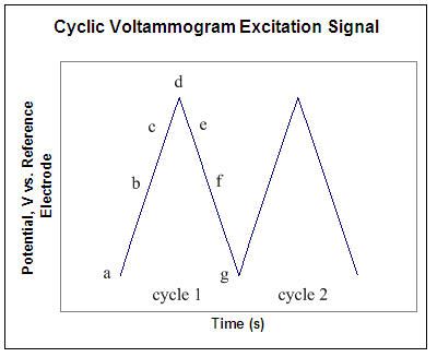
The potential of the working electrode is measured against a reference electrode which maintains a constant potential, and the resulting applied potential produces an excitation signal such as that of figure 1.² In the forward scan of figure 1, the potential first scans negatively, starting from a greater potential (a) and ending at a lower potential (d). The potential extrema (d) is call the switching potential, and is the point where the voltage is sufficient enough to have caused an oxidation or reduction of an analyte. The reverse scan occurs from (d) to (g), and is where the potential scans positively. Figure 1 shows a typical reduction occurring from (a) to (d) and an oxidation occurring from (d) to (g). It is important to note that some analytes undergo oxidation first, in which case the potential would first scan positively. This cycle can be repeated, and the scan rate can be varied. The slope of the excitation signal gives the scan rate used.
A cyclic voltammogram is obtained by measuring the current at the working electrode during the potential scans.² Figure 2 shows a cyclic voltammogram resulting from a single electron reduction and oxidation. Consider the following reversible reaction:
\[M^+ + e^- \rightleftharpoons M \nonumber \]
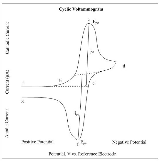
In Figure 2, the reduction process occurs from (a) the initial potential to (d) the switching potential. In this region the potential is scanned negatively to cause a reduction. The resulting current is called cathodic current (ipc). The corresponding peak potential occurs at (c), and is called the cathodic peak potential (Epc). The Epc is reached when all of the substrate at the surface of the electrode has been reduced. After the switching potential has been reached (d), the potential scans positively from (d) to (g). This results in anodic current (Ipa) and oxidation to occur. The peak potential at (f) is called the anodic peak potential (Epa), and is reached when all of the substrate at the surface of the electrode has been oxidized.
Useful Equations for Reversible Systems
Electrode potential (\(E\)):
\[ E = E_i + vt \tag{1} \]
where
- \(E_i\) is the initial potential in volts,
- \(v\) is the sweep rate in volts/s, and
- \(t\) is the time in seconds.
When the direction of the potential sweep is switched, the equation becomes,
\[ E = E_s - vt \tag{2} \]
Where \(E_s\) is the potential at the switching point. Electron stoichiometry (\(n\)):
\[E_p - E_{p/2} > \dfrac{0.0565}{n} \tag{3} \]
where
- \(E_{pa}\) is the anodic peak potential,
- \(E_{pc}\) is the cathodic peak potential, and
- \(n\) is the number of electrons participating in the redox reactions.
Formal Reduction Potential (E°’) is the mean of the \(E_{pc}\) and \(E_{pa}\) values:
\[E°’ = \dfrac{E_{pa} + E_{pc}}{2}. \nonumber \]
Concentration Profiles at the Electrode Surface
In an unstirred solution, mass transport of the analyte to the electrode surface occurs by diffusion alone.¹ Fick’s Law for mass transfer diffusion relates the distance from the electrode (x), time (t), and the reactant concentration (CA) to the diffusion coefficient (DA).
\[ \dfrac{\partial c_A}{\partial t} = D_A \dfrac{\partial^2c_A}{\partial x^2} \tag{4} \]
During a reduction, current increases until it reaches a peak: when all M+ exposed to the surface of an electrode has been reduced to M. At this point additional M+ to be reduced can travel by diffusion alone to the surface of the electrode, and as the concentration of M increases, the distance M+ has to travel also increases. During this process the current which has peaked, begins to decline as smaller and smaller amounts of M+ approach the electrode. It is not practical to obtain limiting currents Ipa, and Ipc in a system in which the electrode has not been stirred because the currents continually decrease with time.¹
In a stirred solution, a Nernst diffusion layer ~10-2 cm thick, lies adjacent to the electrode surface. Beyond this region is a laminar flow region, followed by a turbulent flow region which contains the bulk solution.¹ Because diffusion is limited to the narrow Nernst diffusion region, the reacting analytes cannot diffuse into the bulk solution, and therefore Nernstian equilibrium is maintained and diffusion-controlled currents can be obtained. In this case, Fick’s Law for mass transfer diffusion can be simplified to give the peak current
\[ i_p = (2.69 \; x \; 10^5) \; n^{3/2} \; SD_A^{1/2} \; V^{1/2} \; C_A^* \tag{5} \]
Here, (n) is equal to the number of electrons gained in the reduction, (S) is the surface area of the working electrode in cm², (DA) is the diffusion coefficient, (v) is the sweep rate, and (CA) is the molar concentration of A in the bulk solution.
Instrumentation
A CV system consists of an electrolysis cell, a potentiostat, a current-to-voltage converter, and a data acquisition system. The electrolysis cell consists of a working electrode, counter electrode, reference electrode, and electrolytic solution. The working electrode’s potential is varied linearly with time, while the reference electrode maintains a constant potential. The counter electrode conducts electricity from the signal source to the working electrode. The purpose of the electrolytic solution is to provide ions to the electrodes during oxidation and reduction. A potentiostat is an electronic device which uses a dc power source to produce a potential which can be maintained and accurately determined, while allowing small currents to be drawn into the system without changing the voltage. The current-to-voltage converter measures the resulting current, and the data acquisition system produces the resulting voltammogram.
Applications
Cyclic Voltammetry can be used to study qualitative information about electrochemical processes under various conditions, such as the presence of intermediates in oxidation-reduction reactions, the reversibility of a reaction. CV can also be used to determine the electron stoichiometry of a system, the diffusion coefficient of an analyte, and the formal reduction potential, which can be used as an identification tool. In addition, because concentration is proportional to current in a reversible, Nernstian system, concentration of an unknown solution can be determined by generating a calibration curve of current vs. concentration.
References
- Skoog, D.; Holler, F.; Crouch, S. Principles of Instrumental Analysis 2007
- Kissinger, P. T., Heineman, W. R., “Cyclic Voltammetry,” Journal of Chemical Education, 60, 702 (1983).
- Carriedo, Gabino A. "The use of cyclic voltammetry in the study of the chemistry of metal-carbonyls: An introductory experiment." J. Chem. Educ. 1988, 65, 1020.
Contributors and Attributions
- Amanda Quiroga (UCD)