
30.2: Capillary Electrophoresis
- Page ID
- 362621

\( \newcommand{\vecs}[1]{\overset { \scriptstyle \rightharpoonup} {\mathbf{#1}} } \)
\( \newcommand{\vecd}[1]{\overset{-\!-\!\rightharpoonup}{\vphantom{a}\smash {#1}}} \)
\( \newcommand{\id}{\mathrm{id}}\) \( \newcommand{\Span}{\mathrm{span}}\)
( \newcommand{\kernel}{\mathrm{null}\,}\) \( \newcommand{\range}{\mathrm{range}\,}\)
\( \newcommand{\RealPart}{\mathrm{Re}}\) \( \newcommand{\ImaginaryPart}{\mathrm{Im}}\)
\( \newcommand{\Argument}{\mathrm{Arg}}\) \( \newcommand{\norm}[1]{\| #1 \|}\)
\( \newcommand{\inner}[2]{\langle #1, #2 \rangle}\)
\( \newcommand{\Span}{\mathrm{span}}\)
\( \newcommand{\id}{\mathrm{id}}\)
\( \newcommand{\Span}{\mathrm{span}}\)
\( \newcommand{\kernel}{\mathrm{null}\,}\)
\( \newcommand{\range}{\mathrm{range}\,}\)
\( \newcommand{\RealPart}{\mathrm{Re}}\)
\( \newcommand{\ImaginaryPart}{\mathrm{Im}}\)
\( \newcommand{\Argument}{\mathrm{Arg}}\)
\( \newcommand{\norm}[1]{\| #1 \|}\)
\( \newcommand{\inner}[2]{\langle #1, #2 \rangle}\)
\( \newcommand{\Span}{\mathrm{span}}\) \( \newcommand{\AA}{\unicode[.8,0]{x212B}}\)
\( \newcommand{\vectorA}[1]{\vec{#1}} % arrow\)
\( \newcommand{\vectorAt}[1]{\vec{\text{#1}}} % arrow\)
\( \newcommand{\vectorB}[1]{\overset { \scriptstyle \rightharpoonup} {\mathbf{#1}} } \)
\( \newcommand{\vectorC}[1]{\textbf{#1}} \)
\( \newcommand{\vectorD}[1]{\overrightarrow{#1}} \)
\( \newcommand{\vectorDt}[1]{\overrightarrow{\text{#1}}} \)
\( \newcommand{\vectE}[1]{\overset{-\!-\!\rightharpoonup}{\vphantom{a}\smash{\mathbf {#1}}}} \)
\( \newcommand{\vecs}[1]{\overset { \scriptstyle \rightharpoonup} {\mathbf{#1}} } \)
\( \newcommand{\vecd}[1]{\overset{-\!-\!\rightharpoonup}{\vphantom{a}\smash {#1}}} \)
\(\newcommand{\avec}{\mathbf a}\) \(\newcommand{\bvec}{\mathbf b}\) \(\newcommand{\cvec}{\mathbf c}\) \(\newcommand{\dvec}{\mathbf d}\) \(\newcommand{\dtil}{\widetilde{\mathbf d}}\) \(\newcommand{\evec}{\mathbf e}\) \(\newcommand{\fvec}{\mathbf f}\) \(\newcommand{\nvec}{\mathbf n}\) \(\newcommand{\pvec}{\mathbf p}\) \(\newcommand{\qvec}{\mathbf q}\) \(\newcommand{\svec}{\mathbf s}\) \(\newcommand{\tvec}{\mathbf t}\) \(\newcommand{\uvec}{\mathbf u}\) \(\newcommand{\vvec}{\mathbf v}\) \(\newcommand{\wvec}{\mathbf w}\) \(\newcommand{\xvec}{\mathbf x}\) \(\newcommand{\yvec}{\mathbf y}\) \(\newcommand{\zvec}{\mathbf z}\) \(\newcommand{\rvec}{\mathbf r}\) \(\newcommand{\mvec}{\mathbf m}\) \(\newcommand{\zerovec}{\mathbf 0}\) \(\newcommand{\onevec}{\mathbf 1}\) \(\newcommand{\real}{\mathbb R}\) \(\newcommand{\twovec}[2]{\left[\begin{array}{r}#1 \\ #2 \end{array}\right]}\) \(\newcommand{\ctwovec}[2]{\left[\begin{array}{c}#1 \\ #2 \end{array}\right]}\) \(\newcommand{\threevec}[3]{\left[\begin{array}{r}#1 \\ #2 \\ #3 \end{array}\right]}\) \(\newcommand{\cthreevec}[3]{\left[\begin{array}{c}#1 \\ #2 \\ #3 \end{array}\right]}\) \(\newcommand{\fourvec}[4]{\left[\begin{array}{r}#1 \\ #2 \\ #3 \\ #4 \end{array}\right]}\) \(\newcommand{\cfourvec}[4]{\left[\begin{array}{c}#1 \\ #2 \\ #3 \\ #4 \end{array}\right]}\) \(\newcommand{\fivevec}[5]{\left[\begin{array}{r}#1 \\ #2 \\ #3 \\ #4 \\ #5 \\ \end{array}\right]}\) \(\newcommand{\cfivevec}[5]{\left[\begin{array}{c}#1 \\ #2 \\ #3 \\ #4 \\ #5 \\ \end{array}\right]}\) \(\newcommand{\mattwo}[4]{\left[\begin{array}{rr}#1 \amp #2 \\ #3 \amp #4 \\ \end{array}\right]}\) \(\newcommand{\laspan}[1]{\text{Span}\{#1\}}\) \(\newcommand{\bcal}{\cal B}\) \(\newcommand{\ccal}{\cal C}\) \(\newcommand{\scal}{\cal S}\) \(\newcommand{\wcal}{\cal W}\) \(\newcommand{\ecal}{\cal E}\) \(\newcommand{\coords}[2]{\left\{#1\right\}_{#2}}\) \(\newcommand{\gray}[1]{\color{gray}{#1}}\) \(\newcommand{\lgray}[1]{\color{lightgray}{#1}}\) \(\newcommand{\rank}{\operatorname{rank}}\) \(\newcommand{\row}{\text{Row}}\) \(\newcommand{\col}{\text{Col}}\) \(\renewcommand{\row}{\text{Row}}\) \(\newcommand{\nul}{\text{Nul}}\) \(\newcommand{\var}{\text{Var}}\) \(\newcommand{\corr}{\text{corr}}\) \(\newcommand{\len}[1]{\left|#1\right|}\) \(\newcommand{\bbar}{\overline{\bvec}}\) \(\newcommand{\bhat}{\widehat{\bvec}}\) \(\newcommand{\bperp}{\bvec^\perp}\) \(\newcommand{\xhat}{\widehat{\xvec}}\) \(\newcommand{\vhat}{\widehat{\vvec}}\) \(\newcommand{\uhat}{\widehat{\uvec}}\) \(\newcommand{\what}{\widehat{\wvec}}\) \(\newcommand{\Sighat}{\widehat{\Sigma}}\) \(\newcommand{\lt}{<}\) \(\newcommand{\gt}{>}\) \(\newcommand{\amp}{&}\) \(\definecolor{fillinmathshade}{gray}{0.9}\)Theory of Electrophoresis
In capillary electrophoresis we inject the sample into a buffered solution retained within a capillary tube. When an electric field is applied across the capillary tube, the sample’s components migrate as the result of two types of actions: electrophoretic mobility and electroosmotic mobility. Electrophoretic mobility is the solute’s response to the applied electrical field in which cations move toward the negatively charged cathode, anions move toward the positively charged anode, and neutral species remain stationary. The other contribution to a solute’s migration is electroosmotic flow, which occurs when the buffer moves through the capillary in response to the applied electrical field. Under normal conditions the buffer moves toward the cathode, sweeping most solutes, including the anions and neutral species, toward the negatively charged cathode.
Electrophoretic Mobility
The velocity with which a solute moves in response to the applied electric field is called its electrophoretic velocity, \(\nu_{ep}\); it is defined as
\[\nu_{ep}=\mu_{ep} E \label{12.1} \]
where \(\mu_{ep}\) is the solute’s electrophoretic mobility, and E is the magnitude of the applied electrical field. A solute’s electrophoretic mobility is defined as
\[\mu_{ep}=\frac{q}{6 \pi \eta r} \label{12.2} \]
where q is the solute’s charge, \(\eta\) is the buffer’s viscosity, and r is the solute’s radius. Using Equation \ref{12.1} and Equation \ref{12.2} we can make several important conclusions about a solute’s electrophoretic velocity. Electrophoretic mobility and, therefore, electrophoretic velocity, increases for more highly charged solutes and for solutes of smaller size. Because q is positive for a cation and negative for an anion, these species migrate in opposite directions. A neutral species, for which q is zero, has an electrophoretic velocity of zero.
Electroosmotic Mobility
When an electric field is applied to a capillary filled with an aqueous buffer we expect the buffer’s ions to migrate in response to their electrophoretic mobility. Because the solvent, H2O, is neutral we might reasonably expect it to remain stationary. What we observe under normal conditions, however, is that the buffer moves toward the cathode. This phenomenon is called the electroosmotic flow.
Electroosmotic flow occurs because the walls of the capillary tubing carry a charge. The surface of a silica capillary contains large numbers of silanol groups (–SiOH). At a pH level greater than approximately 2 or 3, the silanol groups ionize to form negatively charged silanate ions (–SiO–). Cations from the buffer are attracted to the silanate ions. As shown in Figure 30.2.1 , some of these cations bind tightly to the silanate ions, forming a fixed layer. Because the cations in the fixed layer only partially neutralize the negative charge on the capillary walls, the solution adjacent to the fixed layer—which is called the diffuse layer—contains more cations than anions. Together these two layers are known as the double layer. Cations in the diffuse layer migrate toward the cathode. Because these cations are solvated, the solution also is pulled along, producing the electroosmotic flow.
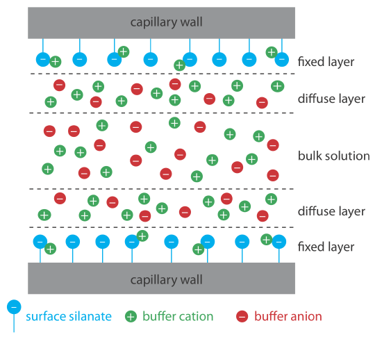
The anions in the diffuse layer, which also are solvated, try to move toward the anode. Because there are more cations than anions, however, the cations win out and the electroosmotic flow moves in the direction of the cathode.
The rate at which the buffer moves through the capillary, what we call its electroosmotic flow velocity, \(\nu_{eof}\), is a function of the applied electric field, E, and the buffer’s electroosmotic mobility, \(\mu_{eof}\).
\[\nu_{eof}=\mu_{e o f} E \label{12.3} \]
Electroosmotic mobility is defined as
\[\mu_{eof}=\frac{\varepsilon \zeta}{4 \pi \eta} \label{12.4} \]
where \(\epsilon\) is the buffer dielectric constant, \(\zeta\) is the zeta potential, and \(\eta\) is the buffer’s viscosity.
The zeta potential—the potential of the diffuse layer at a finite distance from the capillary wall—plays an important role in determining the electroosmotic flow velocity. Two factors determine the zeta potential’s value. First, the zeta potential is directly proportional to the charge on the capillary walls, with a greater density of silanate ions corresponding to a larger zeta potential. Below a pH of 2 there are few silanate ions and the zeta potential and the electroosmotic flow velocity approach zero. As the pH increases, both the zeta potential and the electroosmotic flow velocity increase. Second, the zeta potential is directly proportional to the thickness of the double layer. Increasing the buffer’s ionic strength provides a higher concentration of cations, which decreases the thickness of the double layer and decreases the electroosmotic flow.
The definition of zeta potential given here admittedly is a bit fuzzy. For a more detailed explanation see Delgado, A. V.; González-Caballero, F.; Hunter, R. J.; Koopal, L. K.; Lyklema, J. “Measurement and Interpretation of Electrokinetic Phenomena,” Pure. Appl. Chem. 2005, 77, 1753–1805. Although this is a very technical report, Sections 1.3–1.5 provide a good introduction to the difficulty of defining the zeta potential and of measuring its value.
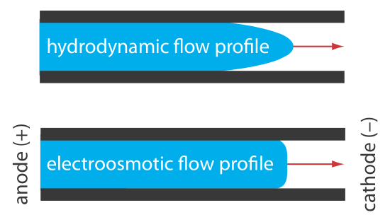
The electroosmotic flow profile is very different from that of a fluid moving under forced pressure. Figure 30.2.2 compares the electroosmotic flow profile with the hydrodynamic flow profile in gas chromatography and liquid chromatography. The uniform, flat profile for electroosmosis helps minimize band broadening in capillary electrophoresis, improving separation efficiency.
Total Mobility
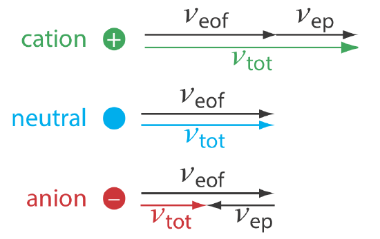
A solute’s total velocity, \(\nu_{tot}\), as it moves through the capillary is the sum of its electrophoretic velocity and the electroosmotic flow velocity.
\[\nu_{t o t}=\nu_{ep}+\nu_{eof} \nonumber \]
As shown in Figure 30.2.3 , under normal conditions the following general relationships hold true.
\[(\nu_{tot})_{cations} > \nu_{eof} \nonumber \]
\[(\nu_{tot})_{neutrals} = \nu_{eof} \nonumber \]
\[(\nu_{tot})_{anions} < \nu_{eof} \nonumber \]
Cations elute first in an order that corresponds to their electrophoretic mobilities, with small, highly charged cations eluting before larger cations of lower charge. Neutral species elute as a single band with an elution rate equal to the electroosmotic flow velocity. Finally, anions are the last components to elute, with smaller, highly charged anions having the longest elution time.
Migration Time
Another way to express a solute’s velocity is to divide the distance it travels by the elapsed time
\[\nu_{tot}=\frac{l}{t_{m}} \label{12.5} \]
where l is the distance between the point of injection and the detector, and tm is the solute’s migration time. To understand the experimental variables that affect migration time, we begin by noting that
\[\nu_{tot} = \mu_{tot}E = (\mu_{ep} + \mu_{eof})E \label{12.6} \]
Combining Equation \ref{12.5} and Equation \ref{12.6} and solving for tm leaves us with
\[t_{\mathrm{m}}=\frac{l}{\left(\mu_{ep}+\mu_{eof}\right) E} \label{12.7} \]
The magnitude of the electrical field is
\[E=\frac{V}{L} \label{12.8} \]
where V is the applied potential and L is the length of the capillary tube. Finally, substituting Equation \ref{12.8} into Equation \ref{12.7} leaves us with the following equation for a solute’s migration time.
\[t_{\mathrm{m}}=\frac{lL}{\left(\mu_{ep}+\mu_{eof}\right) V} \label{12.9} \]
To decrease a solute’s migration time—which shortens the analysis time—we can apply a higher voltage or use a shorter capillary tube. We can also shorten the migration time by increasing the electroosmotic flow, although this decreases resolution.
Efficiency
As we learned in Chapter 26.3, the efficiency of a separation is given by the number of theoretical plates, N. In capillary electrophoresis the number of theoretic plates is
\[N=\frac{l^{2}}{2 D t_{m}}=\frac{\left(\mu_{e p}+\mu_{eof}\right) E l}{2 D L} \label{12.10} \]
where D is the solute’s diffusion coefficient. From Equation \ref{12.10}, the efficiency of a capillary electrophoretic separation increases with higher voltages. Increasing the electroosmotic flow velocity improves efficiency, but at the expense of resolution. Two additional observations deserve comment. First, solutes with larger electrophoretic mobilities—in the same direction as the electroosmotic flow—have greater efficiencies; thus, smaller, more highly charged cations are not only the first solutes to elute, but do so with greater efficiency. Second, efficiency in capillary electrophoresis is independent of the capillary’s length. Theoretical plate counts of approximately 100 000–200 000 are not unusual.
It is possible to design an electrophoretic experiment so that anions elute before cations—more about this later—in which smaller, more highly charged anions elute with greater efficiencies.
Selectivity
In chromatography we defined the selectivity between two solutes as the ratio of their retention factors. In capillary electrophoresis the analogous expression for selectivity is
\[\alpha=\frac{\mu_{ep, 1}}{\mu_{ep, 2}} \nonumber \]
where \(\mu_{ep,1}\) and \(\mu_{ep,2}\) are the electrophoretic mobilities for the two solutes, chosen such that \(\alpha \ge 1\). We can often improve selectivity by adjusting the pH of the buffer solution. For example, \(\text{NH}_4^+\) is a weak acid with a pKa of 9.75. At a pH of 9.75 the concentrations of \(\text{NH}_4^+\) and NH3 are equal. Decreasing the pH below 9.75 increases its electrophoretic mobility because a greater fraction of the solute is present as the cation \(\text{NH}_4^+\). On the other hand, raising the pH above 9.75 increases the proportion of neutral NH3, decreasing its electrophoretic mobility.
Resolution
The resolution between two solutes is
\[R = \frac {0.177(\mu_{ep,2} - \mu_{ep,1})\sqrt{V}} {\sqrt{D(\mu_{avg} + \mu_{eof})}} \label{12.11} \]
where \(\mu_{avg}\) is the average electrophoretic mobility for the two solutes. Increasing the applied voltage and decreasing the electroosmotic flow velocity improves resolution. The latter effect is particularly important. Although increasing electroosmotic flow improves analysis time and efficiency, it decreases resolution.
Instrumentation
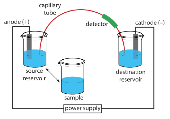
The basic instrumentation for capillary electrophoresis is shown in Figure 30.2.4 and includes a power supply for applying the electric field, anode and cathode compartments that contain reservoirs of the buffer solution, a sample vial that contains the sample, the capillary tube, and a detector. Each part of the instrument receives further consideration in this section.
Capillary Tubes
Figure 30.2.5 shows a cross-section of a typical capillary tube. Most capillary tubes are made from fused silica coated with a 15–35 μm layer of polyimide to give it mechanical strength. The inner diameter is typically 25–75 μm, which is smaller than the internal diameter of a capillary GC column, with an outer diameter of 200–375 μm.
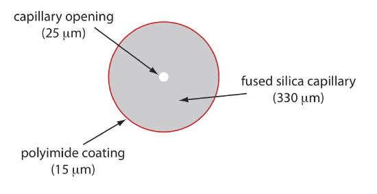
The capillary column’s narrow opening and the thickness of its walls are important. When an electric field is applied to the buffer solution, current flows through the capillary. This current leads to the release of heat, which we call Joule heating. The amount of heat released is proportional to the capillary’s radius and to the magnitude of the electrical field. Joule heating is a problem because it changes the buffer’s viscosity, with the solution at the center of the capillary being less viscous than that near the capillary walls. Because a solute’s electrophoretic mobility depends on its viscosity (see Equation \ref{12.2}), solute species in the center of the capillary migrate at a faster rate than those near the capillary walls. The result is an additional source of band broadening that degrades the separation. Capillaries with smaller inner diameters generate less Joule heating, and capillaries with larger outer diameters are more effective at dissipating the heat. Placing the capillary tube inside a thermostated jacket is another method for minimizing the effect of Joule heating; in this case a smaller outer diameter allows for a more rapid dissipation of thermal energy.
Injecting the Sample
There are two common methods for injecting a sample into a capillary electrophoresis column: hydrodynamic injection and electrokinetic injection. In both methods the capillary tube is filled with the buffer solution. One end of the capillary tube is placed in the destination reservoir and the other end is placed in the sample vial.
Hydrodynamic injection uses pressure to force a small portion of sample into the capillary tubing. A difference in pressure is applied across the capillary either by pressurizing the sample vial or by applying a vacuum to the destination reservoir. The volume of sample injected, in liters, is given by the following equation
\[V_{\text {inj}}=\frac{\Delta P d^{4} \pi t}{128 \eta L} \times 10^{3} \label{12.12} \]
where \(\Delta P\) is the difference in pressure across the capillary in pascals, d is the capillary’s inner diameter in meters, t is the amount of time the pressure is applied in seconds, \(\eta\) is the buffer’s viscosity in kg m–1 s–1, and L is the length of the capillary tubing in meters. The factor of 103 changes the units from cubic meters to liters.
For a hydrodynamic injection we move the capillary from the source reservoir to the sample. The anode remains in the source reservoir. A hydrodynamic injection also is possible if we raise the sample vial above the destination reservoir and briefly insert the filled capillary.
In a hydrodynamic injection we apply a pressure difference of \(2.5 \times 10^3\) Pa (a \(\Delta P \approx 0.02 \text{ atm}\)) for 2 s to a 75-cm long capillary tube with an internal diameter of 50 μm. Assuming the buffer’s viscosity is 10–3 kg m–1 s–1, what volume and length of sample did we inject?
Solution
Making appropriate substitutions into Equation \ref{12.12} gives the sample’s volume as
\[V_{inj}=\frac{\left(2.5 \times 10^{3} \text{ kg} \text{ m}^{-1} \text{ s}^{-2}\right)\left(50 \times 10^{-6} \text{ m}\right)^{4}(3.14)(2 \text{ s})}{(128)\left(0.001 \text{ kg} \text{ m}^{-1} \text{ s}^{-1}\right)(0.75 \text{ m})} \times 10^{3} \mathrm{L} / \mathrm{m}^{3} \nonumber \]
\[V_{inj} = 1 \times 10^{-9} \text{ L} = 1 \text{ nL} \nonumber \]
Because the interior of the capillary is cylindrical, the length of the sample, l, is easy to calculate using the equation for the volume of a cylinder; thus
\[l=\frac{V_{\text {inj}}}{\pi r^{2}}=\frac{\left(1 \times 10^{-9} \text{ L}\right)\left(10^{-3} \text{ m}^{3} / \mathrm{L}\right)}{(3.14)\left(25 \times 10^{-6} \text{ m}\right)^{2}}=5 \times 10^{-4} \text{ m}=0.5 \text{ mm} \nonumber \]
Suppose you need to limit your injection to less than 0.20% of the capillary’s length. Using the information from Example 30.2.1 , what is the maximum injection time for a hydrodynamic injection?
- Answer
-
The capillary is 75 cm long, which means that 0.20% of that sample’s maximum length is 0.15 cm. To convert this to the maximum volume of sample we use the equation for the volume of a cylinder.
\[V_{i n j}=l \pi r^{2}=(0.15 \text{ cm})(3.14)\left(25 \times 10^{-4} \text{ cm}\right)^{2}=2.94 \times 10^{-6} \text{ cm}^{3} \nonumber \]
Given that 1 cm3 is equivalent to 1 mL, the maximum volume is \(2.94 \times 10^{-6}\) mL or \(2.94 \times 10^{-9}\) L. To find the maximum injection time, we first solve Equation \ref{12.12} for t
\[t=\frac{128 V_{inj} \eta L}{P d^{4} \pi} \times 10^{-3} \text{ m}^{3} / \mathrm{L} \nonumber \]
and then make appropriate substitutions.
\[t=\frac{(128)\left(2.94 \times 10^{-9} \text{ L}\right)\left(0.001 \text{ kg } \text{ m}^{-1} \text{ s}^{-1}\right)(0.75 \text{ m})}{\left(2.5 \times 10^{3} \text{ kg } \mathrm{m}^{-1} \text{ s}^{-2}\right)\left(50 \times 10^{-6} \text{ m}\right)^{4}(3.14)} \times \frac{10^{-3} \text{ m}^{3}}{\mathrm{L}} = 5.8 \text{ s} \nonumber \]
The maximum injection time, therefore, is 5.8 s.
In an electrokinetic injection we place both the capillary and the anode into the sample and briefly apply an potential. The volume of injected sample is the product of the capillary’s cross sectional area and the length of the capillary occupied by the sample. In turn, this length is the product of the solute’s velocity (see Equation \ref{12.6}) and time; thus
\[V_{inj} = \pi r^2 L = \pi r^2 (\mu_{ep} + \mu_{eof})E^{\prime}t \label{12.13} \]
where r is the capillary’s radius, L is the capillary’s length, and \(E^{\prime}\) is the effective electric field in the sample. An important consequence of Equation \ref{12.13} is that an electrokinetic injection is biased toward solutes with larger electrophoretic mobilities. If two solutes have equal concentrations in a sample, we inject a larger volume—and thus more moles—of the solute with the larger \(\mu_{ep}\).
The electric field in the sample is different that the electric field in the rest of the capillary because the sample and the buffer have different ionic compositions. In general, the sample’s ionic strength is smaller, which makes its conductivity smaller. The effective electric field is
\[E^{\prime} = E \times \frac {\chi_\text{buffer}} {\chi_\text{sample}}\nonumber \]
where \(\chi_\text{buffer}\) and \(\chi_{sample}\) are the conductivities of the buffer and the sample, respectively.
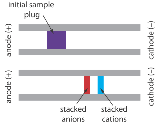
When an analyte’s concentration is too small to detect reliably, it maybe possible to inject it in a manner that increases its concentration. This method of injection is called stacking. Stacking is accomplished by placing the sample in a solution whose ionic strength is significantly less than that of the buffer in the capillary tube. Because the sample plug has a lower concentration of buffer ions, the effective field strength across the sample plug, \(E^{\prime}\), is larger than that in the rest of the capillary.
We know from Equation \ref{12.1} that electrophoretic velocity is directly proportional to the electrical field. As a result, the cations in the sample plug migrate toward the cathode with a greater velocity, and the anions migrate more slowly—neutral species are unaffected and move with the electroosmotic flow. When the ions reach their respective boundaries between the sample plug and the buffer, the electrical field decreases and the electrophoretic velocity of the cations decreases and that for the anions increases. As shown in Figure 30.2.6 , the result is a stacking of cations and anions into separate, smaller sampling zones. Over time, the buffer within the capillary becomes more homogeneous and the separation proceeds without additional stacking.
Applying the Electrical Field
Migration in electrophoresis occurs in response to an applied electric field. The ability to apply a large electric field is important because higher voltages lead to shorter analysis times (Equation \ref{12.9}), more efficient separations (Equation \ref{12.10}), and better resolution (Equation \ref{12.11}). Because narrow bored capillary tubes dissipate Joule heating so efficiently, voltages of up to 40 kV are possible.
Because of the high voltages, be sure to follow your instrument’s safety guidelines.
Detectors
Most of the detectors used in HPLC also find use in capillary electrophoresis. Among the more common detectors are those based on the absorption of UV/Vis radiation, fluorescence, conductivity, amperometry, and mass spectrometry. Whenever possible, detection is done “on-column” before the solutes elute from the capillary tube and additional band broadening occurs.
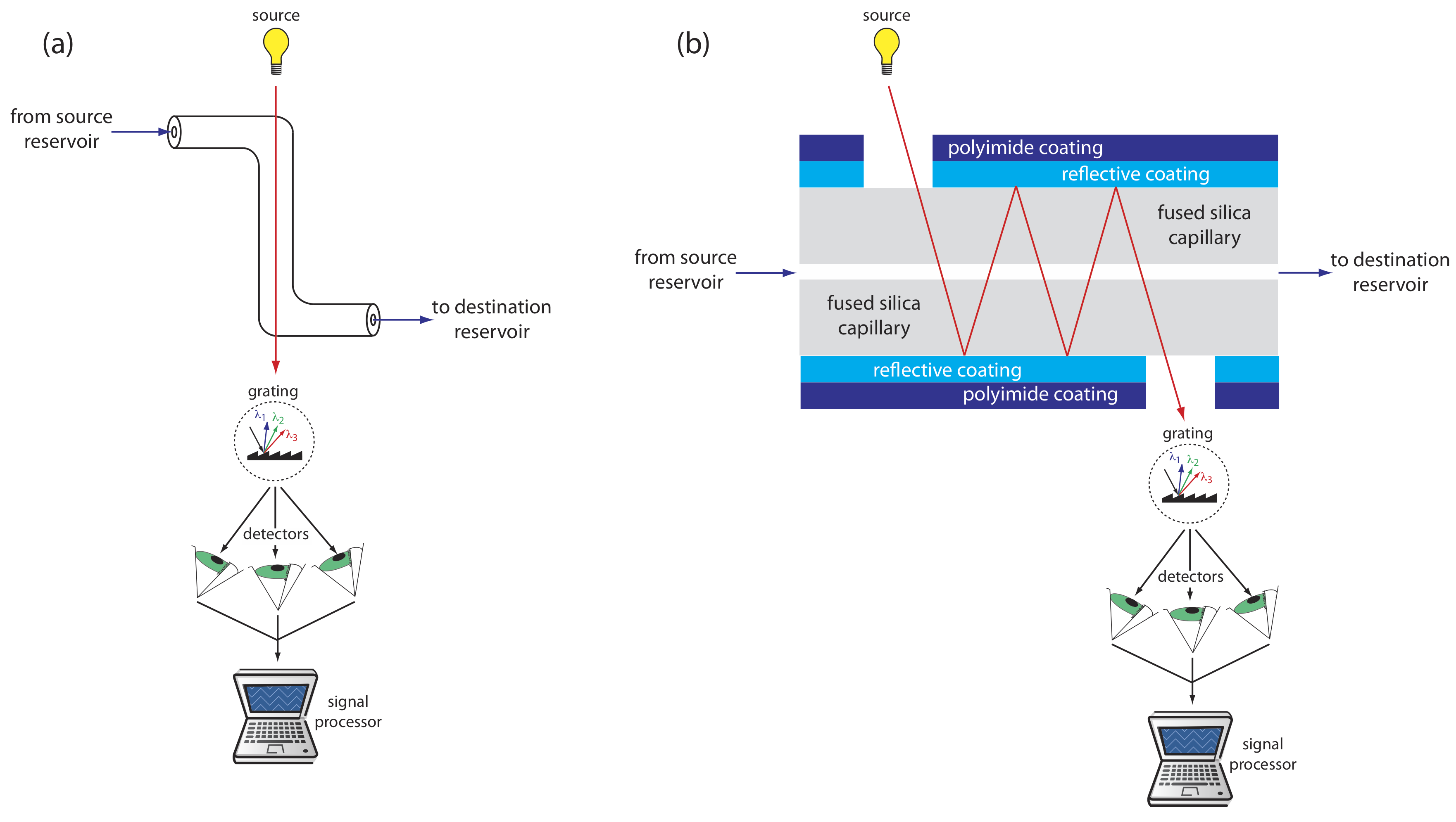
UV/Vis detectors are among the most popular. Because absorbance is directly proportional to path length, the capillary tubing’s small diameter leads to signals that are smaller than those obtained in HPLC. Several approaches have been used to increase the pathlength, including a Z-shaped sample cell and multiple reflections (see Figure 30.2.7 ). Detection limits are about 10–7 M.
Better detection limits are obtained using fluorescence, particularly when using a laser as an excitation source. When using fluorescence detection a small portion of the capillary’s protective coating is removed and the laser beam is focused on the inner portion of the capillary tubing. Emission is measured at an angle of 90o to the laser. Because the laser provides an intense source of radiation that can be focused to a narrow spot, detection limits are as low as 10–16 M.
Solutes that do not absorb UV/Vis radiation or that do not undergo fluorescence can be detected by other detectors. Table 30.2.1 provides a list of detectors for capillary electrophoresis along with some of their important characteristics.
| detector | selectivity (universal or analyte must ...) | detection limited (moles injected) | detection limit (molarity) | on-column detection? |
|---|---|---|---|---|
| UV/Vis absorbance | have a UV/Vis chromophore | \(10^{-13} - 10^{-16}\) | \(10^{-5} - 10^{-7}\) | yes |
| indirect absorbancd | universal | \(10^{-12} - 10^{-15}\) | \(10^{-4} - 10^{-6}\) | yes |
| fluoresence | have a favorable quantum yield | \(10^{-13} - 10^{-17}\) | \(10^{-7} - 10^{-9}\) | yes |
| laser fluorescence | have a favorable quantum yield | \(10^{-18} - 10^{-20}\) | \(10^{-13} - 10^{-16}\) | yes |
| mass spectrometer |
universal (total ion) selective (single ion) |
\(10^{-16} - 10^{-17}\) | \(10^{-8} - 10^{-10}\) | no |
| amperometry | undergo oxidation or reduction | \(10^{-18} - 10^{-19}\) | \(10^{-7} - 10^{-10}\) | no |
| conductivity | universal | \(10^{-15} - 10^{-16}\) | \(10^{-7} - 10^{-9}\) | no |
| radiometric | be radioactive | \(10^{-17} - 10^{-19}\) | \(10^{-10} - 10^{-12}\) | yes |