27.4: Applications of Gas Chromatography

Quantitative Applications

Gas chromatography is widely used for the analysis of a diverse array of samples in environmental, clinical, pharmaceutical, biochemical, forensic, food science and petrochemical laboratories. Table 27.4.1 provides some representative examples of applications.

Table 27.4.1 . Representative Applications of Gas Chromatography

area	applications
environmental analysis	green house gases (CO2, CH4, NOx) in air pesticides in water, wastewater, and soil vehicle emissions trihalomethanes in drinking water
clinical analysis	drugs blood alcohols
forensic analysis	analysis of arson accelerants detection of explosives
consumer products	volatile organics in spices and fragrances trace organics in whiskey monomers in latex paint
petrochemical and chemical industry	purity of solvents refinery gas composition of gasoline

Quantitative Calculations

In a GC analysis the area under the peak is proportional to the amount of analyte injected onto the column. A peak’s area is determined by integration, which usually is handled by the instrument’s computer or by an electronic integrating recorder. If two peak are resolved fully, the determination of their respective areas is straightforward.

Before electronic integrating recorders and computers, two methods were used to find the area under a curve. One method used a manual planimeter; as you use the planimeter to trace an object’s perimeter, it records the area. A second approach for finding a peak’s area is the cut-and-weigh method. The chromatogram is recorded on a piece of paper and each peak of interest is cut out and weighed. Assuming the paper is uniform in thickness and density of fibers, the ratio of weights for two peaks is the same as the ratio of areas. Of course, this approach destroys your chromatogram.

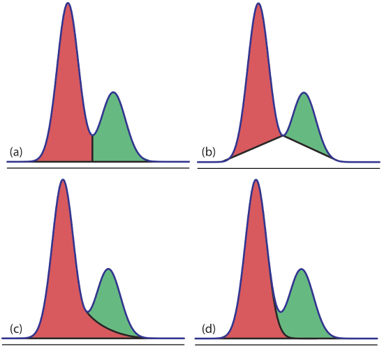
Overlapping peaks, however, require a choice between one of several options for dividing up the area shared by the two peaks (Figure 27.4.1 ). Which method we use depends on the relative size of the two peaks and their resolution. In some cases, the use of peak heights provides more accurate results [(a) Bicking, M. K. L. Chromatography Online, April 2006; (b) Bicking, M. K. L. Chromatography Online, June 2006].

Figure 27.4.1 . Four methods for determining the areas under two overlapping chromatographic peaks: (a) the drop method; (b) the valley method; (c) the exponential skim method; and (d) the Gaussian skim method. Other methods for determining areas also are available.

For quantitative work we need to establish a calibration curve that relates the detector’s response to the analyte’s concentration. If the injection volume is identical for every standard and sample, then an external standardization provides both accurate and precise results. Unfortunately,even under the best conditions the relative precision for replicate injections may differ by 5%; often it is substantially worse. For quantitative work that requires high accuracy and precision, the use of internal standards is recommended.

Example 27.4.1

Marriott and Carpenter report the following data for five replicate injections of a mixture that contains 1% v/v methyl isobutyl ketone and 1% v/v p-xylene in dichloromethane [Marriott, P. J.; Carpenter, P. D. J. Chem. Educ. 1996, 73, 96–99].

injection	peak	peak area (arb. units)
I	1	48075
	2	78112
II	1	85829
	2	135404
III	1	84136
	2	132332
IV	1	71681
	2	112889
V	1	58054
	2	91287

Assume that p-xylene (peak 2) is the analyte, and that methyl isobutyl ketone (peak 1) is the internal standard. Determine the 95% confidence interval for a single-point standardization with and without using the internal standard.

Solution

For a single-point external standardization we ignore the internal standard and determine the relationship between the peak area for p-xylene, A₂, and the concentration, C₂, of p-xylene.

\[A_{2}=k C_{2} \nonumber \]

Substituting the known concentration for p-xylene (1% v/v) and the appropriate peak areas, gives the following values for the constant k.

\[78112 \quad 135404 \quad 132332 \quad 112889 \quad 91287 \nonumber \]

The average value for k is 110 000 with a standard deviation of 25 100 (a relative standard deviation of 22.8%). The 95% confidence interval is

\[\mu=\overline{X} \pm \frac{t s}{\sqrt{n}}=111000 \pm \frac{(2.78)(25100)}{\sqrt{5}}=111000 \pm 31200 \nonumber \]

For an internal standardization, the relationship between the analyte’s peak area, A₂, the internal standard’s peak area, A₁, and their respective concentrations, C₂ and C₁, is

\[\frac{A_{2}}{A_{1}}=k \frac{C_{2}}{C_{1}} \nonumber \]

Substituting in the known concentrations and the appropriate peak areas gives the following values for the constant k.

\[1.5917 \quad 1.5776 \quad 1.5728 \quad 1.5749 \quad 1.5724 \nonumber \]

The average value for k is 1.5779 with a standard deviation of 0.0080 (a relative standard deviation of 0.507%). The 95% confidence interval is

\[\mu=\overline{X} \pm \frac{t s}{\sqrt{n}}=1.5779 \pm \frac{(2.78)(0.0080)}{\sqrt{5}}=1.5779 \pm 0.0099 \nonumber \]

Although there is a substantial variation in the individual peak areas for this set of replicate injections, the internal standard compensates for these variations, providing a more accurate and precise calibration.

Exercise 27.4.1

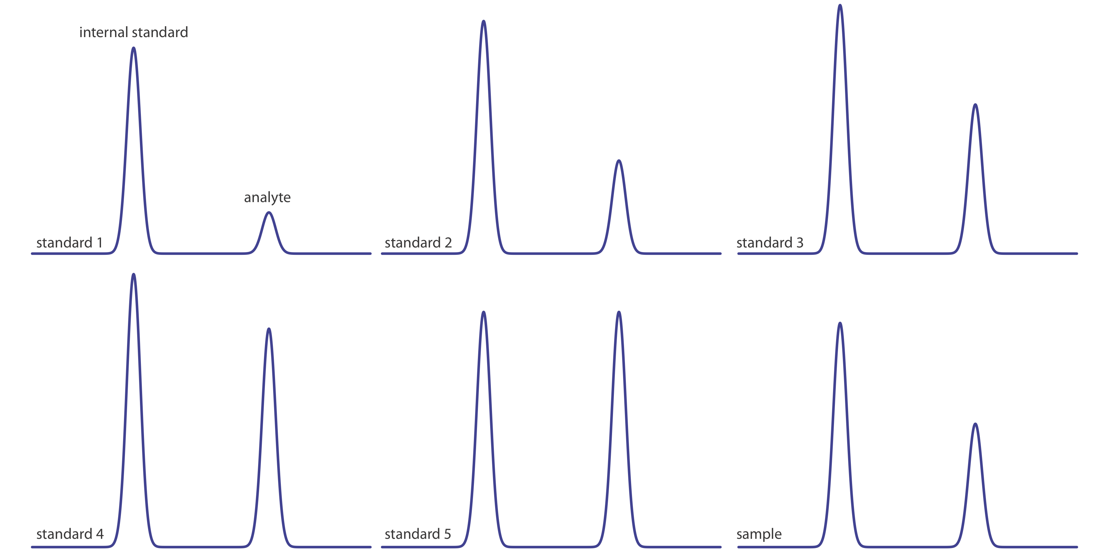
Figure 27.4.2 shows chromatograms for five standards and for one sample. Each standard and sample contains the same concentration of an internal standard, which is 2.50 mg/mL. For the five standards, the concentrations of analyte are 0.20 mg/mL, 0.40 mg/mL, 0.60 mg/mL, 0.80 mg/mL, and 1.00 mg/mL, respectively. Determine the concentration of analyte in the sample by (a) ignoring the internal standards and creating an external standards calibration curve, and by (b) creating an internal standard calibration curve. For each approach, report the analyte’s concentration and the 95% confidence interval. Use peak heights instead of peak areas.

Answer

The following table summarizes my measurements of the peak heights for each standard and the sample, and their ratio (although your absolute values for peak heights will differ from mine, depending on the size of your monitor or printout, your relative peak height ratios should be similar to mine).

[standard] (mg/mL)	peak height of standard (mm)	peak height of analyte (mm)	peak height ratio
0.20	35	7	0.20
0.40	41	16	0.39
0.60	44	27	0.61
0.80	48	39	0.81
1.00	41	41	1.00
sample	39	21	0.54

Figure (a) shows the calibration curve and the calibration equation when we ignore the internal standard. Substituting the sample’s peak height into the calibration equation gives the analyte’s concentration in the sample as 0.49 mg/mL. The 95% confidence interval is ±0.24 mg/mL. The calibration curve shows quite a bit of scatter in the data because of uncertainty in the injection volumes.

Figure (b) shows the calibration curve and the calibration equation when we include the internal standard. Substituting the sample’s peak height ratio into the calibration equation gives the analyte’s concentration in the sample as 0.54 mg/mL. The 95% confidence interval is ±0.04 mg/mL.

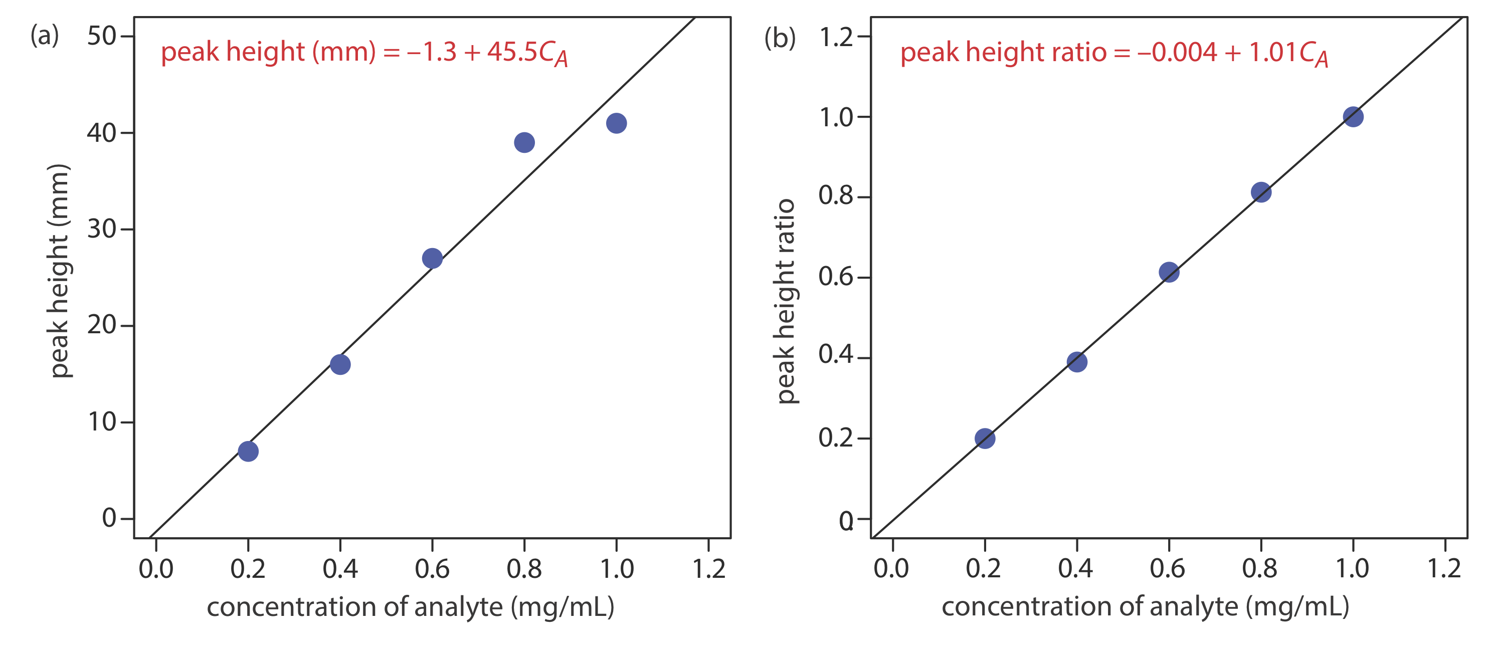
The data for this exercise were created so that the analyte’s actual concentration is 0.55 mg/mL. Given the resolution of my ruler’s scale, my answer is pretty reasonable. Your measurements may be slightly different, but your answers should be close to the actual values.

Figure 27.4.2 . Chromatograms for Exercise 27.4.1.

Qualitative Applications

In addition to a quantitative analysis, we also can use chromatography to identify the components of a mixture. As noted earlier, when we use an FT–IR or a mass spectrometer as the detector we have access to the eluent’s full spectrum for any retention time. By interpreting the spectrum or by searching against a library of spectra, we can identify the analyte responsible for each chromatographic peak.

In addition to identifying the component responsible for a particular chromatographic peak, we also can use the saved spectra to evaluate peak purity. If only one component is responsible for a chromatographic peak, then the spectra should be identical throughout the peak’s elution. If a spectrum at the beginning of the peak’s elution is different from a spectrum taken near the end of the peak’s elution, then at least two components are co-eluting.

When using a nonspectroscopic detector, such as a flame ionization detector, we must find another approach if we wish to identify the components of a mixture. One approach is to spike a sample with the suspected compound and look for an increase in peak height. We also can compare a peak’s retention time to the retention time for a known compound if we use identical operating conditions.

Because a compound’s retention times on two identical columns are not likely to be the same—differences in packing efficiency, for example, will affect a solute’s retention time on a packed column—creating a table of standard retention times is not possible. Kovat’s retention index provides one solution to the problem of matching retention times. Under isothermal conditions, the adjusted retention times for normal alkanes increase logarithmically. Kovat defined the retention index, I, for a normal alkane as 100 times the number of carbon atoms. For example, the retention index is 400 for butane, C₄H₁₀, and 500 for pentane, C₅H₁₂. To determine the a compound’s retention index, I_cpd, we use the following formula

\[I_{cpd} = 100 \times \frac {\log t_{r,cpd}^{\prime} - \log t_{r,x}^{\prime}} {\log t_{r, x+1}^{\prime} - \log t_{r,x}^{\prime}} + I_x \label{12.1} \]

where \(t_{r,cpd}^{\prime}\) is the compound’s adjusted retention time, \(t_{r,x}^{\prime}\) and \(t_{r,x+1}^{\prime}\) are the adjusted retention times for the normal alkanes that elute immediately before the compound and immediately after the compound, respectively, and I_x is the retention index for the normal alkane that elutes immediately before the compound. A compound’s retention index for a particular set of chromatographic conditions—such as the choice of stationary phase, mobile phase, column type, column length, and temperature—is reasonably consistent from day-to-day and between different columns and instruments.

Tables of Kovat’s retention indices are available; see, for example, the NIST Chemistry Webbook. A search for toluene returns 341 values of I for over 20 different stationary phases, and for both packed columns and capillary columns.

Example 27.4.2

In a separation of a mixture of hydrocarbons the following adjusted retention times are measured: 2.23 min for propane, 5.71 min for isobutane, and 6.67 min for butane. What is the Kovat’s retention index for each of these hydrocarbons?

Solution

Kovat’s retention index for a normal alkane is 100 times the number of carbons; thus, for propane, I = 300 and for butane, I = 400. To find Kovat’s retention index for isobutane we use Equation \ref{12.1}.

\[I_\text{isobutane} =100 \times \frac{\log (5.71)-\log (2.23)}{\log (6.67)-\log (2.23)}+300=386 \nonumber \]

Exercise 27.4.2

When using a column with the same stationary phase as in Example 27.4.2 , you find that the retention times for propane and butane are 4.78 min and 6.86 min, respectively. What is the expected retention time for isobutane?

Answer

Because we are using the same column we can assume that isobutane’s retention index of 386 remains unchanged. Using Equation \ref{12.1}, we have

\[386=100 \times \frac{\log x-\log (4.78)}{\log (6.86)-\log (4.78)}+300 \nonumber \]

where x is the retention time for isobutane. Solving for x, we find that

\[0.86=\frac{\log x-\log (4.78)}{\log (6.86)-\log (4.78)} \nonumber \]

\[0.135=\log x-0.679 \nonumber \]

\[0.814=\log x \nonumber \]

\[x=6.52 \nonumber \]

the retention time for isobutane is 6.5 min.