
25.5: Polarography
- Page ID
- 335301

\( \newcommand{\vecs}[1]{\overset { \scriptstyle \rightharpoonup} {\mathbf{#1}} } \)
\( \newcommand{\vecd}[1]{\overset{-\!-\!\rightharpoonup}{\vphantom{a}\smash {#1}}} \)
\( \newcommand{\dsum}{\displaystyle\sum\limits} \)
\( \newcommand{\dint}{\displaystyle\int\limits} \)
\( \newcommand{\dlim}{\displaystyle\lim\limits} \)
\( \newcommand{\id}{\mathrm{id}}\) \( \newcommand{\Span}{\mathrm{span}}\)
( \newcommand{\kernel}{\mathrm{null}\,}\) \( \newcommand{\range}{\mathrm{range}\,}\)
\( \newcommand{\RealPart}{\mathrm{Re}}\) \( \newcommand{\ImaginaryPart}{\mathrm{Im}}\)
\( \newcommand{\Argument}{\mathrm{Arg}}\) \( \newcommand{\norm}[1]{\| #1 \|}\)
\( \newcommand{\inner}[2]{\langle #1, #2 \rangle}\)
\( \newcommand{\Span}{\mathrm{span}}\)
\( \newcommand{\id}{\mathrm{id}}\)
\( \newcommand{\Span}{\mathrm{span}}\)
\( \newcommand{\kernel}{\mathrm{null}\,}\)
\( \newcommand{\range}{\mathrm{range}\,}\)
\( \newcommand{\RealPart}{\mathrm{Re}}\)
\( \newcommand{\ImaginaryPart}{\mathrm{Im}}\)
\( \newcommand{\Argument}{\mathrm{Arg}}\)
\( \newcommand{\norm}[1]{\| #1 \|}\)
\( \newcommand{\inner}[2]{\langle #1, #2 \rangle}\)
\( \newcommand{\Span}{\mathrm{span}}\) \( \newcommand{\AA}{\unicode[.8,0]{x212B}}\)
\( \newcommand{\vectorA}[1]{\vec{#1}} % arrow\)
\( \newcommand{\vectorAt}[1]{\vec{\text{#1}}} % arrow\)
\( \newcommand{\vectorB}[1]{\overset { \scriptstyle \rightharpoonup} {\mathbf{#1}} } \)
\( \newcommand{\vectorC}[1]{\textbf{#1}} \)
\( \newcommand{\vectorD}[1]{\overrightarrow{#1}} \)
\( \newcommand{\vectorDt}[1]{\overrightarrow{\text{#1}}} \)
\( \newcommand{\vectE}[1]{\overset{-\!-\!\rightharpoonup}{\vphantom{a}\smash{\mathbf {#1}}}} \)
\( \newcommand{\vecs}[1]{\overset { \scriptstyle \rightharpoonup} {\mathbf{#1}} } \)
\(\newcommand{\longvect}{\overrightarrow}\)
\( \newcommand{\vecd}[1]{\overset{-\!-\!\rightharpoonup}{\vphantom{a}\smash {#1}}} \)
\(\newcommand{\avec}{\mathbf a}\) \(\newcommand{\bvec}{\mathbf b}\) \(\newcommand{\cvec}{\mathbf c}\) \(\newcommand{\dvec}{\mathbf d}\) \(\newcommand{\dtil}{\widetilde{\mathbf d}}\) \(\newcommand{\evec}{\mathbf e}\) \(\newcommand{\fvec}{\mathbf f}\) \(\newcommand{\nvec}{\mathbf n}\) \(\newcommand{\pvec}{\mathbf p}\) \(\newcommand{\qvec}{\mathbf q}\) \(\newcommand{\svec}{\mathbf s}\) \(\newcommand{\tvec}{\mathbf t}\) \(\newcommand{\uvec}{\mathbf u}\) \(\newcommand{\vvec}{\mathbf v}\) \(\newcommand{\wvec}{\mathbf w}\) \(\newcommand{\xvec}{\mathbf x}\) \(\newcommand{\yvec}{\mathbf y}\) \(\newcommand{\zvec}{\mathbf z}\) \(\newcommand{\rvec}{\mathbf r}\) \(\newcommand{\mvec}{\mathbf m}\) \(\newcommand{\zerovec}{\mathbf 0}\) \(\newcommand{\onevec}{\mathbf 1}\) \(\newcommand{\real}{\mathbb R}\) \(\newcommand{\twovec}[2]{\left[\begin{array}{r}#1 \\ #2 \end{array}\right]}\) \(\newcommand{\ctwovec}[2]{\left[\begin{array}{c}#1 \\ #2 \end{array}\right]}\) \(\newcommand{\threevec}[3]{\left[\begin{array}{r}#1 \\ #2 \\ #3 \end{array}\right]}\) \(\newcommand{\cthreevec}[3]{\left[\begin{array}{c}#1 \\ #2 \\ #3 \end{array}\right]}\) \(\newcommand{\fourvec}[4]{\left[\begin{array}{r}#1 \\ #2 \\ #3 \\ #4 \end{array}\right]}\) \(\newcommand{\cfourvec}[4]{\left[\begin{array}{c}#1 \\ #2 \\ #3 \\ #4 \end{array}\right]}\) \(\newcommand{\fivevec}[5]{\left[\begin{array}{r}#1 \\ #2 \\ #3 \\ #4 \\ #5 \\ \end{array}\right]}\) \(\newcommand{\cfivevec}[5]{\left[\begin{array}{c}#1 \\ #2 \\ #3 \\ #4 \\ #5 \\ \end{array}\right]}\) \(\newcommand{\mattwo}[4]{\left[\begin{array}{rr}#1 \amp #2 \\ #3 \amp #4 \\ \end{array}\right]}\) \(\newcommand{\laspan}[1]{\text{Span}\{#1\}}\) \(\newcommand{\bcal}{\cal B}\) \(\newcommand{\ccal}{\cal C}\) \(\newcommand{\scal}{\cal S}\) \(\newcommand{\wcal}{\cal W}\) \(\newcommand{\ecal}{\cal E}\) \(\newcommand{\coords}[2]{\left\{#1\right\}_{#2}}\) \(\newcommand{\gray}[1]{\color{gray}{#1}}\) \(\newcommand{\lgray}[1]{\color{lightgray}{#1}}\) \(\newcommand{\rank}{\operatorname{rank}}\) \(\newcommand{\row}{\text{Row}}\) \(\newcommand{\col}{\text{Col}}\) \(\renewcommand{\row}{\text{Row}}\) \(\newcommand{\nul}{\text{Nul}}\) \(\newcommand{\var}{\text{Var}}\) \(\newcommand{\corr}{\text{corr}}\) \(\newcommand{\len}[1]{\left|#1\right|}\) \(\newcommand{\bbar}{\overline{\bvec}}\) \(\newcommand{\bhat}{\widehat{\bvec}}\) \(\newcommand{\bperp}{\bvec^\perp}\) \(\newcommand{\xhat}{\widehat{\xvec}}\) \(\newcommand{\vhat}{\widehat{\vvec}}\) \(\newcommand{\uhat}{\widehat{\uvec}}\) \(\newcommand{\what}{\widehat{\wvec}}\) \(\newcommand{\Sighat}{\widehat{\Sigma}}\) \(\newcommand{\lt}{<}\) \(\newcommand{\gt}{>}\) \(\newcommand{\amp}{&}\) \(\definecolor{fillinmathshade}{gray}{0.9}\)The first important voltammetric technique to be developed—polarography—uses the dropping mercury (DME) electrode as the working electrode (see Figure 25.2.2 for a schematic diagram of the DME as well as two other types of Hg electrodes). In polarography, as in linear sweep voltammetry, we vary the potential and measure the current. The change in potential can be in the form of a linear ramp, as was the case for linear sweep voltammetry, or it can involve a series of pulses.
Normal Polarography
As shown in Figure \(\PageIndex{1}\), the current is measured while applying a linear potential ramp.
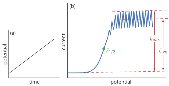
Although polarography takes place in an unstirred solution, we obtain a limiting current instead of a peak current. When a Hg drop separates from the glass capillary and falls to the bottom of the electrochemical cell, it mixes the solution. Each new Hg drop, therefore, grows into a solution whose composition is identical to the bulk solution. The oscillations in the current are a result of the Hg drop’s growth, which leads to a time-dependent change in the area of the working electrode. The limiting current—which also is called the diffusion current—is measured using either the maximum current, imax, or from the average current, iavg. The relationship between the analyte’s concentration, CA, and the limiting current is given by the Ilkovic equations
\[i_{\max }=706 n D^{1 / 2} m^{2 / 3} t^{1 / 6} C_{A}=K_{\max } C_{A} \label{pol1} \]
\[i_{avg}=607 n D^{1 / 2} m^{2 / 3} t^{1 / 6} C_{A}=K_{\mathrm{avg}} C_{A} \label{pol2} \]
where n is the number of electrons in the redox reaction, D is the analyte’s diffusion coefficient, m is the flow rate of Hg, t is the drop’s lifetime and Kmax and Kavg are constants. The half-wave potential, E1/2, provides qualitative information about the redox reaction.
Pulse Polarography
Normal polarography has been replaced by various forms of pulse polarography, several examples of which are shown in Figure \(\PageIndex{2}\) [see Osteryoung, J. J. Chem. Educ. 1983, 60, 296–298 for a comprehensive review]. Normal pulse polarography (Figure \(\PageIndex{2}\)a), for example, uses a series of potential pulses characterized by a cycle of time \(\tau\), a pulse-time of tp, a pulse potential of \(\Delta E_\text{p}\), and a scan rate of \(\Delta E/ \Delta t\). Typical experimental conditions for normal pulse polarography are \(\tau \approx 1 \text{ s}\), tp ≈ 50 ms, and \(\Delta E/ \Delta t \approx 2 \text{ mV/s}\). The initial value of \(\Delta E_\text{p} \approx 2 \text{ mV}\), and it increases by ≈ 2 mV with each pulse. The current is sampled at the end of each potential pulse for approximately 17 ms before returning the potential to its initial value. The shape of the resulting voltammogram is similar to Figure \(\PageIndex{1}\), but without the current oscillations. Because we apply the potential for only a small portion of the drop’s lifetime, there is less time for the analyte to undergo oxidation or reduction and a smaller diffusion layer. As a result, the faradaic current in normal pulse polarography is greater than in the polarography, resulting in better sensitivity and smaller detection limits.

In differential pulse polarography (Figure \(\PageIndex{2}\)b) the current is measured twice per cycle: for approximately 17 ms before applying the pulse and for approximately 17 ms at the end of the cycle. The difference in the two currents gives rise to the peak-shaped voltammogram. Typical experimental conditions for differential pulse polarography are \(\tau \approx 1 \text{ s}\), tp ≈ 50 ms, \(\Delta E_\text{p}\) ≈ 50 mV, and \(\Delta E/ \Delta t\) ≈ 2 mV/s.
The voltammogram for differential pulse polarography is approximately the first derivative of the voltammogram for normal pulse polarography. To see why this is the case, note that the change in current over a fixed change in potential, \(\Delta i / \Delta E\), approximates the slope of the voltammogram for normal pulse polarography. You may recall that the first derivative of a function returns the slope of the function at each point. The first derivative of a sigmoidal function is a peak-shaped function.
Other forms of pulse polarography include staircase polarography (Figure \(\PageIndex{2}\)c) and square-wave polarography (Figure \(\PageIndex{2}\)d). One advantage of square-wave polarography is that we can make \(\tau\) very small—perhaps as small as 5 ms, compared to 1 s for other forms of pulse polarography—which significantly decreases analysis time. For example, suppose we need to scan a potential range of 400 mV. If we use normal pulse polarography with a \(\Delta E/ \Delta t\) of 2 mV/cycle and a \(\tau\) of 1 s/cycle, then we need 200 s to complete the scan. If we use square-wave polarography with a \(\Delta E/ \Delta t\) of 2 mV/cycle and a \(\tau\) of 5 ms/cycle, we can complete the scan in 1 s. At this rate, we can acquire a complete voltammogram using a single drop of Hg!
Applications
Polarography is used extensively for the analysis of metal ions and inorganic anions, such as \(\text{IO}_3^-\) and \(\text{NO}_3^-\). We also can use polarography to study organic compounds with easily reducible or oxidizable functional groups, such as carbonyls, carboxylic acids, and carbon-carbon double bonds.