
24.3: Controlled-Current Coulometry
- Page ID
- 333856

\( \newcommand{\vecs}[1]{\overset { \scriptstyle \rightharpoonup} {\mathbf{#1}} } \)
\( \newcommand{\vecd}[1]{\overset{-\!-\!\rightharpoonup}{\vphantom{a}\smash {#1}}} \)
\( \newcommand{\dsum}{\displaystyle\sum\limits} \)
\( \newcommand{\dint}{\displaystyle\int\limits} \)
\( \newcommand{\dlim}{\displaystyle\lim\limits} \)
\( \newcommand{\id}{\mathrm{id}}\) \( \newcommand{\Span}{\mathrm{span}}\)
( \newcommand{\kernel}{\mathrm{null}\,}\) \( \newcommand{\range}{\mathrm{range}\,}\)
\( \newcommand{\RealPart}{\mathrm{Re}}\) \( \newcommand{\ImaginaryPart}{\mathrm{Im}}\)
\( \newcommand{\Argument}{\mathrm{Arg}}\) \( \newcommand{\norm}[1]{\| #1 \|}\)
\( \newcommand{\inner}[2]{\langle #1, #2 \rangle}\)
\( \newcommand{\Span}{\mathrm{span}}\)
\( \newcommand{\id}{\mathrm{id}}\)
\( \newcommand{\Span}{\mathrm{span}}\)
\( \newcommand{\kernel}{\mathrm{null}\,}\)
\( \newcommand{\range}{\mathrm{range}\,}\)
\( \newcommand{\RealPart}{\mathrm{Re}}\)
\( \newcommand{\ImaginaryPart}{\mathrm{Im}}\)
\( \newcommand{\Argument}{\mathrm{Arg}}\)
\( \newcommand{\norm}[1]{\| #1 \|}\)
\( \newcommand{\inner}[2]{\langle #1, #2 \rangle}\)
\( \newcommand{\Span}{\mathrm{span}}\) \( \newcommand{\AA}{\unicode[.8,0]{x212B}}\)
\( \newcommand{\vectorA}[1]{\vec{#1}} % arrow\)
\( \newcommand{\vectorAt}[1]{\vec{\text{#1}}} % arrow\)
\( \newcommand{\vectorB}[1]{\overset { \scriptstyle \rightharpoonup} {\mathbf{#1}} } \)
\( \newcommand{\vectorC}[1]{\textbf{#1}} \)
\( \newcommand{\vectorD}[1]{\overrightarrow{#1}} \)
\( \newcommand{\vectorDt}[1]{\overrightarrow{\text{#1}}} \)
\( \newcommand{\vectE}[1]{\overset{-\!-\!\rightharpoonup}{\vphantom{a}\smash{\mathbf {#1}}}} \)
\( \newcommand{\vecs}[1]{\overset { \scriptstyle \rightharpoonup} {\mathbf{#1}} } \)
\(\newcommand{\longvect}{\overrightarrow}\)
\( \newcommand{\vecd}[1]{\overset{-\!-\!\rightharpoonup}{\vphantom{a}\smash {#1}}} \)
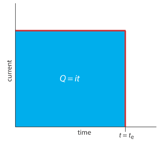
\(\newcommand{\avec}{\mathbf a}\) \(\newcommand{\bvec}{\mathbf b}\) \(\newcommand{\cvec}{\mathbf c}\) \(\newcommand{\dvec}{\mathbf d}\) \(\newcommand{\dtil}{\widetilde{\mathbf d}}\) \(\newcommand{\evec}{\mathbf e}\) \(\newcommand{\fvec}{\mathbf f}\) \(\newcommand{\nvec}{\mathbf n}\) \(\newcommand{\pvec}{\mathbf p}\) \(\newcommand{\qvec}{\mathbf q}\) \(\newcommand{\svec}{\mathbf s}\) \(\newcommand{\tvec}{\mathbf t}\) \(\newcommand{\uvec}{\mathbf u}\) \(\newcommand{\vvec}{\mathbf v}\) \(\newcommand{\wvec}{\mathbf w}\) \(\newcommand{\xvec}{\mathbf x}\) \(\newcommand{\yvec}{\mathbf y}\) \(\newcommand{\zvec}{\mathbf z}\) \(\newcommand{\rvec}{\mathbf r}\) \(\newcommand{\mvec}{\mathbf m}\) \(\newcommand{\zerovec}{\mathbf 0}\) \(\newcommand{\onevec}{\mathbf 1}\) \(\newcommand{\real}{\mathbb R}\) \(\newcommand{\twovec}[2]{\left[\begin{array}{r}#1 \\ #2 \end{array}\right]}\) \(\newcommand{\ctwovec}[2]{\left[\begin{array}{c}#1 \\ #2 \end{array}\right]}\) \(\newcommand{\threevec}[3]{\left[\begin{array}{r}#1 \\ #2 \\ #3 \end{array}\right]}\) \(\newcommand{\cthreevec}[3]{\left[\begin{array}{c}#1 \\ #2 \\ #3 \end{array}\right]}\) \(\newcommand{\fourvec}[4]{\left[\begin{array}{r}#1 \\ #2 \\ #3 \\ #4 \end{array}\right]}\) \(\newcommand{\cfourvec}[4]{\left[\begin{array}{c}#1 \\ #2 \\ #3 \\ #4 \end{array}\right]}\) \(\newcommand{\fivevec}[5]{\left[\begin{array}{r}#1 \\ #2 \\ #3 \\ #4 \\ #5 \\ \end{array}\right]}\) \(\newcommand{\cfivevec}[5]{\left[\begin{array}{c}#1 \\ #2 \\ #3 \\ #4 \\ #5 \\ \end{array}\right]}\) \(\newcommand{\mattwo}[4]{\left[\begin{array}{rr}#1 \amp #2 \\ #3 \amp #4 \\ \end{array}\right]}\) \(\newcommand{\laspan}[1]{\text{Span}\{#1\}}\) \(\newcommand{\bcal}{\cal B}\) \(\newcommand{\ccal}{\cal C}\) \(\newcommand{\scal}{\cal S}\) \(\newcommand{\wcal}{\cal W}\) \(\newcommand{\ecal}{\cal E}\) \(\newcommand{\coords}[2]{\left\{#1\right\}_{#2}}\) \(\newcommand{\gray}[1]{\color{gray}{#1}}\) \(\newcommand{\lgray}[1]{\color{lightgray}{#1}}\) \(\newcommand{\rank}{\operatorname{rank}}\) \(\newcommand{\row}{\text{Row}}\) \(\newcommand{\col}{\text{Col}}\) \(\renewcommand{\row}{\text{Row}}\) \(\newcommand{\nul}{\text{Nul}}\) \(\newcommand{\var}{\text{Var}}\) \(\newcommand{\corr}{\text{corr}}\) \(\newcommand{\len}[1]{\left|#1\right|}\) \(\newcommand{\bbar}{\overline{\bvec}}\) \(\newcommand{\bhat}{\widehat{\bvec}}\) \(\newcommand{\bperp}{\bvec^\perp}\) \(\newcommand{\xhat}{\widehat{\xvec}}\) \(\newcommand{\vhat}{\widehat{\vvec}}\) \(\newcommand{\uhat}{\widehat{\uvec}}\) \(\newcommand{\what}{\widehat{\wvec}}\) \(\newcommand{\Sighat}{\widehat{\Sigma}}\) \(\newcommand{\lt}{<}\) \(\newcommand{\gt}{>}\) \(\newcommand{\amp}{&}\) \(\definecolor{fillinmathshade}{gray}{0.9}\)A second approach to coulometry is to use a constant current in place of a constant potential, which results in the current-versus-time profile shown in Figure \(\PageIndex{1}\). Controlled-current coulometry has two advantages over controlled-potential coulometry. First, the analysis time is shorter because the current does not decrease over time. A typical analysis time for controlled-current coulometry is less than 10 min, compared to approximately 30–60 min for controlled-potential coulometry. Second, because the total charge is simply the product of current and time, there is no need to integrate the current-time curve in Figure \(\PageIndex{1}\).
Using a constant current presents us with two important experimental problems. First, during electrolysis the analyte’s concentration—and, therefore, the current that results from its oxidation or reduction—decreases continuously. To maintain a constant current we must allow the potential to change until another oxidation reaction or reduction reaction occurs at the working electrode. Unless we design the system carefully, this secondary reaction results in a current efficiency that is less than 100%. The second problem is that we need a method to determine when the analyte's electrolysis is complete. In a controlled-potential coulometric analysis we know that electrolysis is complete when the current reaches zero, or when it reaches a constant background or residual current. In a controlled-current coulometric analysis, however, current continues to flow even when the analyte’s electrolysis is complete. A suitable method for determining the reaction’s endpoint, te, is needed.
Maintaining Current Efficiency
To illustrate why a change in the working electrode’s potential may result in a current efficiency of less than 100%, let’s consider the coulometric analysis for Fe2+ based on its oxidation to Fe3+ at a Pt working electrode in 1 M H2SO4.
\[\mathrm{Fe}^{2+}(a q) \rightleftharpoons \text{ Fe}^{3+}(a q)+e^{-} \label{ci1} \]
Figure \(\PageIndex{2}\) shows the relevant potentials for this system. At the beginning of the analysis, the potential of the working electrode remains nearly constant at a level near its initial value.
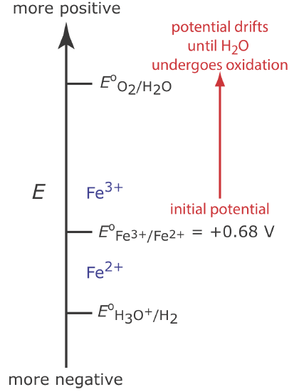
As the concentration of Fe2+ decreases and the concentration of Fe3+ increases, the working electrode’s potential shifts toward more positive values until the oxidation of H2O begins.
\[2 \mathrm{H}_{2} \mathrm{O}(l)\rightleftharpoons \text{ O}_{2}(g)+4 \mathrm{H}^{+}(a q)+4 e^{-} \label{ci2} \]
Because a portion of the total current comes from the oxidation of H2O, the current efficiency for the analysis is less than 100% and we cannot use the equation \(Q = it\) to determine the amount of Fe2+ in the sample.
Although we cannot prevent the potential from drifting until another species undergoes oxidation, we can maintain a 100% current efficiency if the product of that secondary oxidation reaction both rapidly and quantitatively reacts with the remaining Fe2+. To accomplish this we add an excess of Ce3+ to the analytical solution. As shown in Figure \(\PageIndex{3}\), when the potential of the working electrode shifts to a more positive potential, Ce3+ begins to oxidize to Ce4+
\[\mathrm{Ce}^{3+}(a q) \rightleftharpoons \text{ Ce}^{4+}(a q)+e^{-} \label{ci3} \]
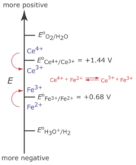
The Ce4+ that forms at the working electrode rapidly mixes with the solution where it reacts with any available Fe2+.
\[\mathrm{Ce}^{4+}(a q)+\text{ Fe}^{2+}(a q) \rightleftharpoons \text{ Ce}^{3+}(a q)+\text{ Fe}^{3+}(a q) \label{ci4} \]
Combining reaction \ref{ci3} and reaction \ref{ci4} shows that the net reaction is the oxidation of Fe2+ to Fe3+
\[\mathrm{Fe}^{2+}(a q) \rightleftharpoons \text{ Fe}^{3+}(a q)+e^{-} \label{ci5} \]
which maintains a current efficiency of 100%. A species used to maintain 100% current efficiency is called a mediator.
Endpoint Determination
Adding a mediator solves the problem of maintaining 100% current efficiency, but it does not solve the problem of determining when the analyte's electrolysis is complete. Using the analysis for Fe2+ in Figure \(\PageIndex{3}\), when the oxidation of Fe2+ is complete current continues to flow from the oxidation of Ce3+, and, eventually, the oxidation of H2O. What we need is a signal that tells us when no more Fe2+ is present in the solution.
For our purposes, it is convenient to treat a controlled-current coulometric analysis as a reaction between the analyte, Fe2+, and the mediator, Ce3+, as shown by reaction \ref{ci4}. This reaction is identical to a redox titration; thus, we can use the end points for a redox titration—visual indicators and potentiometric or conductometric measurements—to signal the end of a controlled-current coulometric analysis. For example, ferroin provides a useful visual endpoint for the Ce3+ mediated coulometric analysis for Fe2+, changing color from red to blue when the electrolysis of Fe2+ is complete.
Instrumentation
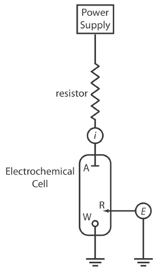
We can carry out controlled-current coulometry using the two-electrode galvanostat shown in Figure \(\PageIndex{4}\), which consists of a working electrode and a counter electrode. The working electrode—often a simple Pt electrode—also is called the generator electrode since it is where the mediator reacts to generate the species that reacts with the analyte. If necessary, the counter electrode is isolated from the analytical solution by a salt bridge or a porous frit to prevent its electrolysis products from reacting with the analyte. The current from the power supply through the working electrode is
\[i=\frac{E_{\mathrm{PS}}}{R+R_{\mathrm{cell}}} \label{ci6} \]
where EPS is the potential of the power supply, R is the resistance of the resistor, and Rcell is the resistance of the electrochemical cell. If R >> Rcell, then the current between the auxiliary and working electrodes
\[i=\frac{E_{\mathrm{PS}}}{R} \approx \text{constant} \label{ci7} \]
maintains a constant value. To monitor the working electrode’s potential, which changes as the composition of the electrochemical cell changes, we can include an optional reference electrode and a high-impedance potentiometer.
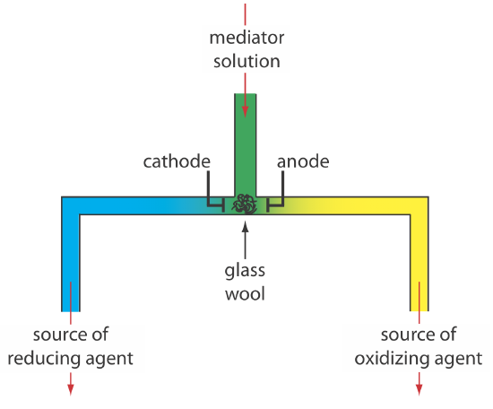
Alternatively, we can generate the oxidizing agent or the reducing agent externally, and allow it to flow into the analytical solution. Figure \(\PageIndex{5}\) shows one simple method for accomplishing this. A solution that contains the mediator flows into a small-volume electrochemical cell with the products exiting through separate tubes. Depending upon the analyte, the oxidizing agent or the reducing reagent is delivered to the analytical solution. For example, we can generate Ce4+ using an aqueous solution of Ce3+, directing the Ce4+ that forms at the anode to our sample.
There are two other crucial needs for controlled-current coulometry: an accurate clock for measuring the electrolysis time, te, and a switch for starting and stopping the electrolysis. An analog clock can record time to the nearest ±0.01 s, but the need to stop and start the electrolysis as we approach the endpoint may result in an overall uncertainty of ±0.1 s. A digital clock allows for a more accurate measurement of time, with an overall uncertainty of ±1 ms. The switch must control both the current and the clock so that we can make an accurate determination of the electrolysis time.
Coulometric Titrations
A controlled-current coulometric method sometimes is called a coulometric titration because of its similarity to a conventional titration. For example, in the controlled-current coulometric analysis for Fe2+ using a Ce3+ mediator, the oxidation of Fe2+ by Ce4+ (reaction \ref{ci4}) is identical to the reaction in a redox titration.
There are other similarities between controlled-current coulometry and titrimetry. If we combine the equation \(Q = nFN_a\) and the equation \(Q = it_e\) and solve for the moles of analyte, NA, we obtain the following equation.
\[N_{A}=\frac{i}{n F} \times t_{e} \label{ci8} \]
Compare Equation \ref{ci8} to the relationship between the moles of analyte, NA, and the moles of titrant, NT, in a titration
\[N_{A}=N_{T}=M_{T} \times V_{T} \label{ci9} \]
where MT and VT are the titrant’s molarity and the volume of titrant at the end point. In constant-current coulometry, the current source is equivalent to the titrant and the value of that current is analogous to the titrant’s molarity. Electrolysis time is analogous to the volume of titrant, and te is equivalent to the a titration’s end point. Finally, the switch for starting and stopping the electrolysis serves the same function as a buret’s stopcock.
For simplicity, we assumed above that the stoichiometry between the analyte and titrant is 1:1. The assumption, however, is not important and does not effect our observation of the similarity between controlled-current coulometry and a titration.
Quantitative Applications
The use of a mediator makes a coulometric titration a more versatile analytical technique than controlled-potential coulometry. For example, the direct oxidation or reduction of a protein at a working electrode is difficult if the protein’s active redox site lies deep within its structure. A coulometric titration of the protein is possible, however, if we use the oxidation or reduction of a mediator to produce a solution species that reacts with the protein. Table \(\PageIndex{1}\) summarizes several controlled-current coulometric methods based on a redox reaction using a mediator.
For an analyte that is not easy to oxidize or reduce, we can complete a coulometric titration by coupling a mediator’s oxidation or reduction to an acid–base, precipitation, or complexation reaction that involves the analyte. For example, if we use H2O as a mediator, we can generate H3O+at the anode
\[6 \mathrm{H}_{2} \mathrm{O}(l) \rightleftharpoons 4 \mathrm{H}_{3} \text{O}^{+}(a q)+\text{ O}_{2}(g)+4 e^{-} \nonumber \]
and generate OH– at the cathode.
\[2 \mathrm{H}_{2} \mathrm{O}(l)+2 e^{-} \rightleftharpoons 2 \mathrm{OH}^{-}(a q)+\text{ H}_{2}(g) \nonumber \]
If we carry out the oxidation or reduction of H2O using the generator cell in Figure \(\PageIndex{5}\), then we can selectively dispense H3O+ or OH– into a solution that contains the analyte. The resulting reaction is identical to that in an acid–base titration. Coulometric acid–base titrations have been used for the analysis of strong and weak acids and bases, in both aqueous and non-aqueous matrices. Table \(\PageIndex{2}\) summarizes several examples of coulometric titrations that involve acid–base, complexation, and precipitation reactions.
In comparison to a conventional titration, a coulometric titration has two important advantages. The first advantage is that electrochemically generating a titrant allows us to use a reagent that is unstable. Although we cannot prepare and store a solution of a highly reactive reagent, such as Ag2+ or Mn3+, we can generate them electrochemically and use them in a coulometric titration. Second, because it is relatively easy to measure a small quantity of charge, we can use a coulometric titration to determine an analyte whose concentration is too small for a conventional titration.
The following example shows the calculations for a typical coulometric analysis.
To determine the purity of a sample of Na2S2O3, a sample is titrated coulometrically using I– as a mediator and \(\text{I}_3^-\) as the titrant. A sample weighing 0.1342 g is transferred to a 100-mL volumetric flask and diluted to volume with distilled water. A 10.00-mL portion is transferred to an electrochemical cell along with 25 mL of 1 M KI, 75 mL of a pH 7.0 phosphate buffer, and several drops of a starch indicator solution. Electrolysis at a constant current of 36.45 mA requires 221.8 s to reach the starch indicator endpoint. Determine the sample’s purity.
Solution
As shown in Table \(\PageIndex{1}\), the coulometric titration of \(\text{S}_2 \text{O}_3^{2-}\) with \(\text{I}_3^-\) is
\[2 \mathrm{S}_{2} \mathrm{O}_{3}^{2-}(a q)+\text{ I}_{3}^{-}(a q)\rightleftharpoons \text{ S}_{4} \mathrm{O}_{6}^{2-}(a q)+3 \mathrm{I}^{-}(a q) \nonumber \]
The oxidation of \(\text{S}_2 \text{O}_3^{2-}\) to \(\text{S}_4 \text{O}_6^{2-}\) requires one electron per \(\text{S}_2 \text{O}_3^{2-}\) (n = 1). Combining the equations \(Q = nFN_A\) and \(Q = it_e\), and solving for the moles and grams of Na2S2O3 gives
\[N_{A} =\frac{i t_{e}}{n F}=\frac{(0.03645 \text{ A})(221.8 \text{ s})}{\left(\frac{1 \text{ mol } e^{-}}{\text{mol Na}_{2} \mathrm{S}_{2} \mathrm{O}_{3}}\right)\left(\frac{96487 \text{ C}}{\text{mol } e^{-}}\right)} =8.379 \times 10^{-5} \text{ mol Na}_{2} \mathrm{S}_{2} \mathrm{O}_{3} \nonumber \]
This is the amount of Na2S2O3 in a 10.00-mL portion of a 100-mL sample; thus, there are 0.1325 grams of Na2S2O3 in the original sample. The sample’s purity, therefore, is
\[\frac{0.1325 \text{ g} \text{ Na}_{2} \mathrm{S}_{2} \mathrm{O}_{3}}{0.1342 \text{ g} \text { sample }} \times 100=98.73 \% \text{ w} / \text{w } \mathrm{Na}_{2} \mathrm{S}_{2} \mathrm{O}_{3} \nonumber \]
Note that for this calcuation, it does not matter whether \(\text{S}_2 \text{O}_3^{2-}\) is oxidized at the working electrode or is oxidized by \(\text{I}_3^-\).