24.2: Controlled-Potential Coulometry
- Page ID
- 333854

\( \newcommand{\vecs}[1]{\overset { \scriptstyle \rightharpoonup} {\mathbf{#1}} } \)
\( \newcommand{\vecd}[1]{\overset{-\!-\!\rightharpoonup}{\vphantom{a}\smash {#1}}} \)
\( \newcommand{\id}{\mathrm{id}}\) \( \newcommand{\Span}{\mathrm{span}}\)
( \newcommand{\kernel}{\mathrm{null}\,}\) \( \newcommand{\range}{\mathrm{range}\,}\)
\( \newcommand{\RealPart}{\mathrm{Re}}\) \( \newcommand{\ImaginaryPart}{\mathrm{Im}}\)
\( \newcommand{\Argument}{\mathrm{Arg}}\) \( \newcommand{\norm}[1]{\| #1 \|}\)
\( \newcommand{\inner}[2]{\langle #1, #2 \rangle}\)
\( \newcommand{\Span}{\mathrm{span}}\)
\( \newcommand{\id}{\mathrm{id}}\)
\( \newcommand{\Span}{\mathrm{span}}\)
\( \newcommand{\kernel}{\mathrm{null}\,}\)
\( \newcommand{\range}{\mathrm{range}\,}\)
\( \newcommand{\RealPart}{\mathrm{Re}}\)
\( \newcommand{\ImaginaryPart}{\mathrm{Im}}\)
\( \newcommand{\Argument}{\mathrm{Arg}}\)
\( \newcommand{\norm}[1]{\| #1 \|}\)
\( \newcommand{\inner}[2]{\langle #1, #2 \rangle}\)
\( \newcommand{\Span}{\mathrm{span}}\) \( \newcommand{\AA}{\unicode[.8,0]{x212B}}\)
\( \newcommand{\vectorA}[1]{\vec{#1}} % arrow\)
\( \newcommand{\vectorAt}[1]{\vec{\text{#1}}} % arrow\)
\( \newcommand{\vectorB}[1]{\overset { \scriptstyle \rightharpoonup} {\mathbf{#1}} } \)
\( \newcommand{\vectorC}[1]{\textbf{#1}} \)
\( \newcommand{\vectorD}[1]{\overrightarrow{#1}} \)
\( \newcommand{\vectorDt}[1]{\overrightarrow{\text{#1}}} \)
\( \newcommand{\vectE}[1]{\overset{-\!-\!\rightharpoonup}{\vphantom{a}\smash{\mathbf {#1}}}} \)
\( \newcommand{\vecs}[1]{\overset { \scriptstyle \rightharpoonup} {\mathbf{#1}} } \)
\( \newcommand{\vecd}[1]{\overset{-\!-\!\rightharpoonup}{\vphantom{a}\smash {#1}}} \)
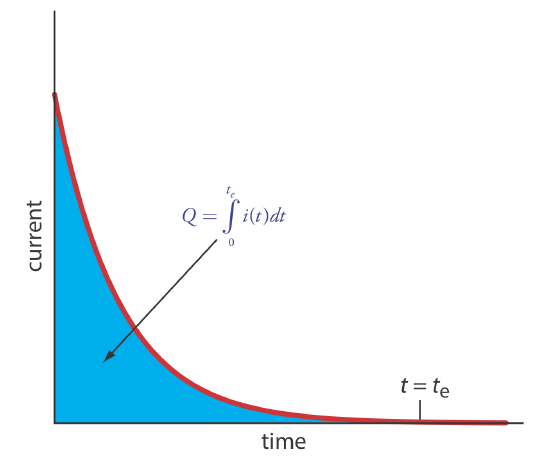
\(\newcommand{\avec}{\mathbf a}\) \(\newcommand{\bvec}{\mathbf b}\) \(\newcommand{\cvec}{\mathbf c}\) \(\newcommand{\dvec}{\mathbf d}\) \(\newcommand{\dtil}{\widetilde{\mathbf d}}\) \(\newcommand{\evec}{\mathbf e}\) \(\newcommand{\fvec}{\mathbf f}\) \(\newcommand{\nvec}{\mathbf n}\) \(\newcommand{\pvec}{\mathbf p}\) \(\newcommand{\qvec}{\mathbf q}\) \(\newcommand{\svec}{\mathbf s}\) \(\newcommand{\tvec}{\mathbf t}\) \(\newcommand{\uvec}{\mathbf u}\) \(\newcommand{\vvec}{\mathbf v}\) \(\newcommand{\wvec}{\mathbf w}\) \(\newcommand{\xvec}{\mathbf x}\) \(\newcommand{\yvec}{\mathbf y}\) \(\newcommand{\zvec}{\mathbf z}\) \(\newcommand{\rvec}{\mathbf r}\) \(\newcommand{\mvec}{\mathbf m}\) \(\newcommand{\zerovec}{\mathbf 0}\) \(\newcommand{\onevec}{\mathbf 1}\) \(\newcommand{\real}{\mathbb R}\) \(\newcommand{\twovec}[2]{\left[\begin{array}{r}#1 \\ #2 \end{array}\right]}\) \(\newcommand{\ctwovec}[2]{\left[\begin{array}{c}#1 \\ #2 \end{array}\right]}\) \(\newcommand{\threevec}[3]{\left[\begin{array}{r}#1 \\ #2 \\ #3 \end{array}\right]}\) \(\newcommand{\cthreevec}[3]{\left[\begin{array}{c}#1 \\ #2 \\ #3 \end{array}\right]}\) \(\newcommand{\fourvec}[4]{\left[\begin{array}{r}#1 \\ #2 \\ #3 \\ #4 \end{array}\right]}\) \(\newcommand{\cfourvec}[4]{\left[\begin{array}{c}#1 \\ #2 \\ #3 \\ #4 \end{array}\right]}\) \(\newcommand{\fivevec}[5]{\left[\begin{array}{r}#1 \\ #2 \\ #3 \\ #4 \\ #5 \\ \end{array}\right]}\) \(\newcommand{\cfivevec}[5]{\left[\begin{array}{c}#1 \\ #2 \\ #3 \\ #4 \\ #5 \\ \end{array}\right]}\) \(\newcommand{\mattwo}[4]{\left[\begin{array}{rr}#1 \amp #2 \\ #3 \amp #4 \\ \end{array}\right]}\) \(\newcommand{\laspan}[1]{\text{Span}\{#1\}}\) \(\newcommand{\bcal}{\cal B}\) \(\newcommand{\ccal}{\cal C}\) \(\newcommand{\scal}{\cal S}\) \(\newcommand{\wcal}{\cal W}\) \(\newcommand{\ecal}{\cal E}\) \(\newcommand{\coords}[2]{\left\{#1\right\}_{#2}}\) \(\newcommand{\gray}[1]{\color{gray}{#1}}\) \(\newcommand{\lgray}[1]{\color{lightgray}{#1}}\) \(\newcommand{\rank}{\operatorname{rank}}\) \(\newcommand{\row}{\text{Row}}\) \(\newcommand{\col}{\text{Col}}\) \(\renewcommand{\row}{\text{Row}}\) \(\newcommand{\nul}{\text{Nul}}\) \(\newcommand{\var}{\text{Var}}\) \(\newcommand{\corr}{\text{corr}}\) \(\newcommand{\len}[1]{\left|#1\right|}\) \(\newcommand{\bbar}{\overline{\bvec}}\) \(\newcommand{\bhat}{\widehat{\bvec}}\) \(\newcommand{\bperp}{\bvec^\perp}\) \(\newcommand{\xhat}{\widehat{\xvec}}\) \(\newcommand{\vhat}{\widehat{\vvec}}\) \(\newcommand{\uhat}{\widehat{\uvec}}\) \(\newcommand{\what}{\widehat{\wvec}}\) \(\newcommand{\Sighat}{\widehat{\Sigma}}\) \(\newcommand{\lt}{<}\) \(\newcommand{\gt}{>}\) \(\newcommand{\amp}{&}\) \(\definecolor{fillinmathshade}{gray}{0.9}\)The easiest way to ensure 100% current efficiency is to hold the working electrode at a constant potential where the analyte is oxidized or reduced completely and where no potential interfering species are oxidized or reduced. As electrolysis progresses, the analyte’s concentration and the current decrease. The resulting current-versus-time profile for controlled-potential coulometry is shown in Figure \(\PageIndex{1}\). Integrating the area under the curve from t = 0 to t = te gives the total charge. In this section we consider the experimental parameters and instrumentation needed to develop a controlled-potential coulometric method of analysis and its applications.
Selecting a Constant Potential
To understand how an appropriate potential for the working electrode is selected, let’s develop a constant-potential coulometric method for Cu2+ based on its reduction to copper metal at a Pt working electrode.
\[\mathrm{Cu}^{2+}(a q)+2 e^{-} \rightleftharpoons \mathrm{Cu}(s) \label{cp1} \]
Figure \(\PageIndex{2}\) shows the three reduction reactions that can take place in an aqueous solution of Cu2+ and their standard state reduction potentials: the reduction of O2 to H2O, the reduction of Cu2+ to Cu, and the reduction of H3O+ to H2. From the diagram we know that reaction \ref{cp1} is favored when the working electrode’s potential is more negative than +0.342 V versus the standard hydrogen electrode. To ensure a 100% current efficiency, however, the potential must be sufficiently more positive than +0.000 V so that the reduction of H3O+ to H2 does not contribute significantly to the total current flowing through the electrochemical cell.
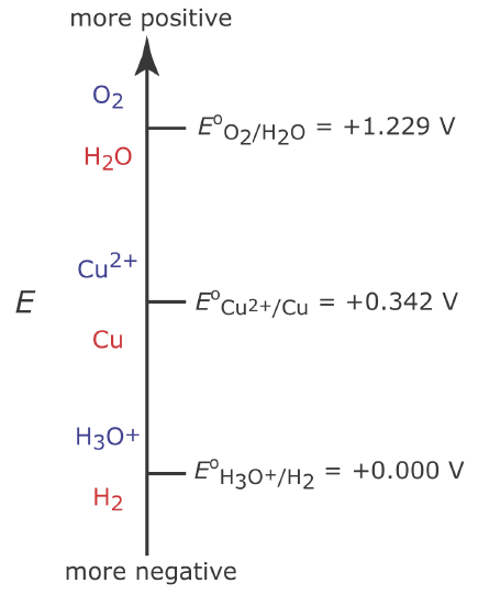
We can use the Nernst equation for reaction \ref{cp1} to estimate the minimum potential for quantitatively reducing Cu2+.
\[E=E_{\mathrm{Cu}^{2+} / \mathrm{Cu}}^{\mathrm{o}}-\frac{0.05916}{2} \log \frac{1}{\left[\mathrm{Cu}^{2+}\right]} \label{cp2} \]
So why are we using the concentration of Cu2+ in Equation \ref{cp2} instead of its activity as we did in Chapter 23 when we considered potentiometry? In potentiometry we used activity because we used Ecell to determine the analyte’s concentration. Here we use the Nernst equation to help us select an appropriate potential. Once we identify a potential, we can adjust its value as needed to ensure a quantitative reduction of Cu2+. In addition, in coulometry the analyte’s concentration is given by the total charge, not the applied potential.
If we define a quantitative electrolysis as one in which we reduce 99.99% of Cu2+ to Cu, then the concentration of Cu2+ at te is
\[\left[\mathrm{Cu}^{2+}\right]_{t_{e}}=0.0001 \times\left[\mathrm{Cu}^{2+}\right]_{0} \label{cp3} \]
where [Cu2+]0 is the initial concentration of Cu2+ in the sample. Substituting Equation \ref{cp3} into Equation \ref{cp2} allows us to calculate the desired potential.
\[E=E_{\mathrm{Cu}^{2+} / \mathrm{Cu}}^{\circ}-\frac{0.05916}{2} \log \frac{1}{0.0001 \times\left[\mathrm{Cu}^{2+}\right]} \label{cp4} \]
If the initial concentration of Cu2+ is \(1.00 \times 10^{-4}\) M, for example, then the working electrode’s potential must be more negative than +0.105 V to quantitatively reduce Cu2+ to Cu. Note that at this potential H3O+ is not reduced to H2, maintaining 100% current efficiency.
Many controlled-potential coulometric methods for Cu2+ use a potential that is negative relative to the standard hydrogen electrode—see, for example, Rechnitz, G. A. Controlled-Potential Analysis, Macmillan: New York, 1963, p.49. Based on Figure \(\PageIndex{2}\) you might expect that applying a potential <0.000 V will partially reduce H3O+ to H2, resulting in a current efficiency that is less than 100%. The reason we can use such a negative potential is that the reaction rate for the reduction of H3O+ to H2 is very slow at a Pt electrode. This results in a significant overpotential—the need to apply a potential more positive or a more negative than that predicted by thermodynamics—which shifts Eo for the H3O+/H2 redox couple to a more negative value.
Minimizing Electrolysis Time
In controlled-potential coulometry, as shown in Figure \(\PageIndex{1}\), the current decreases over time. As a result, the rate of electrolysis—recall from Chapter 22 that current is a measure of rate—becomes slower and an exhaustive electrolysis of the analyte may require a long time. Because time is an important consideration when designing an analytical method, we need to consider the factors that affect the analysis time.
We can approximate how the current changes as a function of time (Figure \(\PageIndex{1}\)) as an exponential decay; thus, the current at time t is
\[i_{t}=i_{0} e^{-k t} \label{cp5} \]
where i0 is the current at t = 0 and k is a rate constant that is directly proportional to the area of the working electrode and the rate of stirring, and that is inversely proportional to the volume of solution. For an exhaustive electrolysis in which we oxidize or reduce 99.99% of the analyte, the current at the end of the analysis, te, is
\[i_{t_{e}} \leq 0.0001 \times i_{0} \label{cp6} \]
Substituting Equation \ref{cp6} into Equation \ref{cp5} and solving for te gives the minimum time for an exhaustive electrolysis as
\[t_{e}=-\frac{1}{k} \times \ln (0.0001)=\frac{9.21}{k} \label{cp7} \]
From this equation we see that a larger value for k reduces the analysis time. For this reason we usually carry out a controlled-potential coulometric analysis in a small volume electrochemical cell, using an electrode with a large surface area, and with a high stirring rate. A quantitative electrolysis typically requires approximately 30–60 min, although shorter or longer times are possible.
Instrumentation
We can use the three-electrode potentiostat in Figure (\(\PageIndex{3}\)) to set and control the potential in controlled-potential coulometry . The potential of the working electrode is measured relative to a constant-potential reference electrode that is connected to the working electrode through a high-impedance potentiometer. To set the working electrode’s potential we adjust the slide wire resistor that is connected to the auxiliary electrode. If the working electrode’s potential begins to drift, we adjust the slide wire resistor to return the potential to its initial value. The current flowing between the auxiliary electrode and the working electrode is measured with an ammeter. Of course, a modern potentionstat uses operational amplifiers to maintain the constant potential without our intervention.
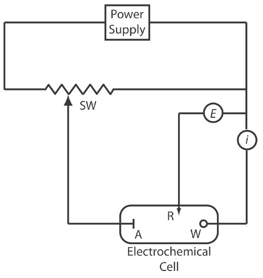
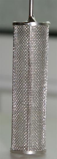
The working electrode is usually one of two types: a cylindrical Pt electrode manufactured from platinum-gauze (Figure \(\PageIndex{4}\)), or a Hg pool electrode. The large overpotential for the reduction of H3O+ at Hg makes it the electrode of choice for an analyte that requires a negative potential. For example, a potential more negative than –1 V versus the SHE is feasible at a Hg electrode—but not at a Pt electrode—even in a very acidic solution. Because mercury is easy to oxidize, it is less useful if we need to maintain a potential that is positive with respect to the SHE. Platinum is the working electrode of choice when we need to apply a positive potential.
The auxiliary electrode, which often is a Pt wire, is separated by a salt bridge from the analytical solution. This is necessary to prevent the electrolysis products generated at the auxiliary electrode from reacting with the analyte and interfering in the analysis. A saturated calomel or Ag/AgCl electrode serves as the reference electrode.
The other essential need for controlled-potential coulometry is a means for determining the total charge. One method is to monitor the current as a function of time and determine the area under the curve, as shown in Figure \(\PageIndex{1}\). Modern instruments use electronic integration to monitor charge as a function of time. The total charge at the end of the electrolysis is read directly from a digital readout.
Electrogravimetry
If the product of controlled-potential coulometry forms a deposit on the working electrode, then we can use the change in the electrode’s mass as the analytical signal. For example, if we apply a potential that reduces Cu2+ to Cu at a Pt working electrode, the difference in the electrode’s mass before and after electrolysis is a direct measurement of the amount of copper in the sample. An analytical technique that uses mass as a signal a gravimetric technique; thus, we call this electrogravimetry.
Quantitative Applications
The majority of controlled-potential coulometric analyses involve the determination of inorganic cations and anions, including trace metals and halides ions. Table \(\PageIndex{1}\) summarizes several of these methods.
| analyte | electrolytic reaction | electrode |
|---|---|---|
| antimony | \(\text{Sb}(\text{III}) + 3 e^{-} \rightleftharpoons \text{Sb}\) | Pt |
| arsenic | \(\text{As}(\text{III}) \rightleftharpoons \text{As(V)} + 2 e^{-}\) | Pt |
| cadmium | \(\text{Cd(II)} + 2 e^{-} \rightleftharpoons \text{Cd}\) | Pt or Hg |
| cobalt | \(\text{Co(II)} + 2 e^{-} \rightleftharpoons \text{Co}\) | Pt or Hg |
| copper | \(\text{Cu(II)} + 2 e^{-} \rightleftharpoons \text{Cu}\) | Pt or Hg |
| halides (X–) | \(\text{Ag} + \text{X}^- \rightleftharpoons \text{AgX} + e^-\) | Ag |
| iron | \(\text{Fe(II)} \rightleftharpoons \text{Fe(III)} + e^-\) | Pt |
| lead | \(\text{Pb(II)} + 2 e^{-} \rightleftharpoons \text{Pb}\) | Pt or Hg |
| nickel | \(\text{Ni(II)} + 2 e^{-} \rightleftharpoons \text{Ni}\) | Pt or Hg |
| plutonium | \(\text{Pu(III)} \rightleftharpoons \text{Pu(IV)} + e^-\) | Pt |
| silver | \(\text{Ag(I)} + 1 e^{-} \rightleftharpoons \text{Ag}\) | Pt |
| tin | \(\text{Sn(II)} + 2 e^{-} \rightleftharpoons \text{Sn}\) | Pt |
| uranium | \(\text{U(VI)} + 2 e^{-} \rightleftharpoons \text{U(IV})\) | Pt or Hg |
| zinc | \(\text{Zn(II)} + 2 e^{-} \rightleftharpoons \text{Zn}\) | Pt or Hg |
|
Source: Rechnitz, G. A. Controlled-Potential Analysis, Macmillan: New York, 1963. Electrolytic reactions are written in terms of the change in the analyte’s oxidation state. The actual species in solution depends on the analyte. |
||
The ability to control selectivity by adjusting the working electrode’s potential makes controlled-potential coulometry particularly useful for the analysis of alloys. For example, we can determine the composition of an alloy that contains Ag, Bi, Cd, and Sb by dissolving the sample and placing it in a matrix of 0.2 M H2SO4 along with a Pt working electrode and a Pt counter electrode. If we apply a constant potential of +0.40 V versus the SCE, Ag(I) deposits on the electrode as Ag and the other metal ions remain in solution. When electrolysis is complete, we use the total charge to determine the amount of silver in the alloy. Next, we shift the working electrode’s potential to –0.08 V versus the SCE, depositing Bi on the working electrode. When the coulometric analysis for bismuth is complete, we determine antimony by shifting the working electrode’s potential to –0.33 V versus the SCE, depositing Sb. Finally, we determine cadmium following its electrodeposition on the working electrode at a potential of –0.80 V versus the SCE.
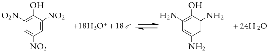
We also can use controlled-potential coulometry for the quantitative analysis of organic compounds, although the number of applications is significantly less than that for inorganic analytes. One example is the six-electron reduction of a nitro group, –NO2, to a primary amine, –NH2, at a mercury electrode. Solutions of picric acid—also known as 2,4,6-trinitrophenol, or TNP, a close relative of TNT—is analyzed by reducing it to triaminophenol.
Another example is the successive reduction of trichloroacetate to dichloroacetate, and of dichloroacetate to monochloroacetate
\[\text{Cl}_3\text{CCOO}^-(aq) + \text{H}_3\text{O}^+(aq) + 2 e^- \rightleftharpoons \text{Cl}_2\text{HCCOO}^-(aq) + \text{Cl}^-(aq) + \text{H}_2\text{O}(l) \nonumber \]
\[\text{Cl}_2\text{HCCOO}^-(aq) + \text{ H}_3\text{O}^+(aq) + 2 e^- \rightleftharpoons \text{ ClH}_2\text{CCOO}^-(aq) + \text{ Cl}^-(aq) + \text{H}_2\text{O}(l) \nonumber \]
We can analyze a mixture of trichloroacetate and dichloroacetate by selecting an initial potential where only the more easily reduced trichloroacetate reacts. When its electrolysis is complete, we can reduce dichloroacetate by adjusting the potential to a more negative potential. The total charge for the first electrolysis gives the amount of trichloroacetate, and the difference in total charge between the first electrolysis and the second electrolysis gives the amount of dichloroacetate.
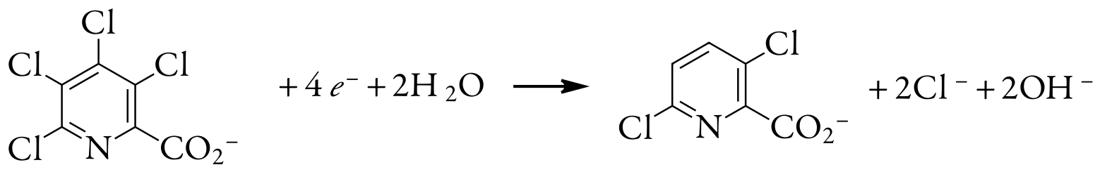
One useful application of controlled-potential coulometry is determining the number of electrons involved in a redox reaction. To make the determination, we complete a controlled-potential coulometric analysis using a known amount of a pure compound. The total charge at the end of the electrolysis is used to determine the value of n using Faraday’s law. A 0.3619-g sample of tetrachloropicolinic acid, C6HNO2Cl4, is dissolved in distilled water, transferred to a 1000-mL volumetric flask, and diluted to volume. An exhaustive controlled-potential electrolysis of a 10.00-mL portion of this solution at a spongy silver cathode requires 5.374 C of charge. What is the value of n for this reduction reaction?
Solution
The 10.00-mL portion of sample contains 3.619 mg, or \(1.39 \times 10^{-5}\) mol of tetrachloropicolinic acid. Solving for n gives
\[n=\frac{Q}{F N_{A}}=\frac{5.374 \text{ C}}{\left(96478 \text{ C/mol } e^{-}\right)\left(1.39 \times 10^{-5} \text{ mol } \mathrm{C}_{6} \mathrm{HNO}_{2} \mathrm{Cl}_{4}\right)} = 4.01 \text{ mol e}^-/\text{mol } \mathrm{C}_{6} \mathrm{HNO}_{2} \mathrm{Cl}_{4} \nonumber \]
Thus, reducing a molecule of tetrachloropicolinic acid requires four electrons. The overall reaction, which results in the selective formation of 3,6-dichloropicolinic acid, is