22.3: Electrode Potentials

We began this chapter by examining the electrochemical cell in Figure 22.1.1 where \(\ce{Zn(s)}\) is oxidized to \(\ce{Zn^{2+}(aq)}\) and \(\ce{Ag^{+}(aq)}\) is reduced to \(\ce{Ag(s)}\), as shown by the following reaction.

\[2 \mathrm{Ag}(s)+\mathrm{Zn}^{2+}(\mathrm{aq}) \rightleftharpoons \mathrm{Zn}(s)+2 \mathrm{Ag}^{+}(a q) \nonumber \]

The reaction proceeds as written because the reduction of Ag⁺(aq) to Ag(s)

\[\mathrm{Ag}^{+}(a q)+e^{-} \rightleftharpoons \mathrm{Ag}(s) \label{red_ag} \]

is more thermodynamically favorable than the reduction of \(\ce{Zn^{2+}(aq)}\) to \(\ce{Zn(s)}\)

\[\text{ Zn}^{2+}(aq)+2 e^{-} \rightleftharpoons \mathrm{Zn}(s) \label{red_zn} \]

But, how do we know this is true? In this section we answer this question by taking a close look at electrode potentials.

Nature of Electrode Potentials

The potential of an electrochemical cell is the difference between the potential at the cathode, \(E_\text{cathode}\), and the potential at the anode, \(E_\text{anode}\), where both potentials are defined in terms of a reduction reaction (and are called reduction potentials); thus

\[E_\text{cell} = E_\text{cathode} - E_\text{anode} \label{cell_pot} \]

\[\mathrm{H}^{+}(a q)+e^{-}=\frac{1}{2} \mathrm{H}_{2}(g) \label{she} \]

which is the reaction that defines the standard hydrogen electrode, or SHE.

The Standard Hydrogen Electrode (SHE)

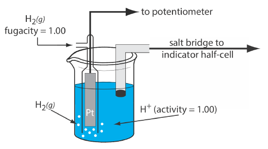
The SHE consists of a Pt electrode immersed in a solution in which the activity of hydrogen ion is 1.00 and in which the partial pressure of H₂(g) is 1.00 atm (Figure \(\PageIndex{1}\)). A conventional salt bridge connects the SHE to the indicator half-cell. The short hand notation for the standard hydrogen electrode is

\[\text{Pt}(s), \text{ H}_{2}\left(g, f_{\mathrm{H}_{2}}=1.00\right) | \text{ H}^{+}\left(a q, a_{\mathrm{H}^{+}}=1.00\right) \| \label{she_cell} \]

and the standard-state potential for the reaction \ref{she} is, by definition, 0.000 V at all temperatures.

Figure \(\PageIndex{1}\). Schematic diagram showing the standard hydrogen electrode.

Practical Reference Electrodes

Although the standard hydrogen electrode is the standard against which all other potentials are referenced, it is not practical for routine use as it is difficult to prepare and maintain. Instead, we use one of several other reference electrodes. The two most common of these alternative reference electrodes are the calomel, or Hg/Hg₂Cl₂ electrode, which is based on the following redox couple between Hg₂Cl₂ and Hg (calomel is the common name for Hg₂Cl₂)

\[\mathrm{Hg}_{2} \mathrm{Cl}_{2}(s)+2 e^{-}\rightleftharpoons2 \mathrm{Hg}(l)+2 \mathrm{Cl}^{-}(a q) \nonumber \]

and the Ag/AgCl reference electrode, which is based on the reduction of AgCl to Ag

\[\operatorname{AgCl}(s)+e^{-} \rightleftharpoons \mathrm{Ag}(s)+\mathrm{Cl}^{-}(a q) \nonumber \]

A more detailed examination of these two reference electrodes is found in Chapter 23.1.

Definition of Electrode Potential

To determine the potential for the reduction of Zn²⁺(aq) to Zn(s) we make it the cathode in the following electrochemical cell

\[\text{Pt}(s), \text{ H}_{2}\left(g, P_{\mathrm{H}_{2}}=1.00\right) | \text{ H}^{+}\left(a q, a_{\mathrm{H}^{+}}=1.00\right) \| \ce{Zn^{2+}}\left(a q, a_{\mathrm{Zn}^{2+}}=x\right) | \ce{Zn}(s) \label{she_zn} \]

where x is the activity of Zn²⁺ in its half-cell. For example, when \(a_{\mathrm{Zn}^{2+}} = 1.00\), the potential of the electrochemical cell is \(-0.763 \text{V}\). If we find that the potential for the electrochemical cell

\[\ce{Zn}(s) | \ce{Zn^{2+}} (aq, a_{\mathrm{Zn}^{2+}} = 1.00) \| \ce{Ag+} (aq, a_{\mathrm{Ag}^{+}} = 1.00) | \ce{Ag}(s) \nonumber \]

is +1.562 V, then knowing that

\[E_{cell} = E_{\ce{Ag+} / \ce{Ag}} - E_{\ce{Zn^{2+}} / \ce{Zn}} = E_{\ce{Ag+} / \ce{Ag}} - (-0.763 \text{V}) \nonumber \]

gives \(E_{\ce{Ag+} / \ce{Ag}} = +0.799\). In this way, we can build tables of potentials for individual half-reactions.

Sign Convention for Electrode Potentials

In Section 22.2 we noted the following relationship between an electrochemical potential, \(E\), and the Gibbs free energy, \(\Delta G\)

\[\Delta G = - n F E \label{dg} \]

which tells us that a positive potential corresponds to a thermodynamically favorable reaction. Knowing that the potential for the electrochemical cell in Equation \ref{she_zn} is \(-0.763 \text{V}\) tells us that the reduction of Zn²⁺(aq) to Zn(s) is not thermodynamically favorable relative to the reduction of H⁺(aq) to H₂(g); that is, we do not expect the reaction

\[\ce{Zn^{2+}}(aq) + \ce{H2}(g) \rightleftharpoons 2 \ce{H+}(aq) + \ce{Zn}(s) \label{zn_h} \]

to occur; however, with a potential of +0.799 V, we do expect the reaction

\[2 \ce{Ag+}(aq) + \ce{H2}(g) \rightleftharpoons 2 \ce{H+}(aq) + 2 \ce{Ag}(s) \label{ag_h} \]

to occur. Or, looking at this another way, we expect that Zn(s), but not Ag(s), will dissolve in acid.

Effect of Activity on Electrode Potentials

In Chapter 22.2 we wrote the Nernst equation for the reaction

\[\mathrm{Zn}(s)+2 \mathrm{Ag}^{+}(a q) \rightleftharpoons 2 \mathrm{Ag}(s)+\mathrm{Zn}^{2+}(\mathrm{aq}) \label{net_rxn} \]

in terms of the concentrations of Zn²⁺(aq) and Ag⁺(aq)

\[E = E^{\circ} - \frac{0.05916}{2} \log \frac {\left[ \ce{Zn^{2+}} \right]} {\left[ \ce{Ag+} \right]^2} \label{zn_ag_conc} \]

Although there are times when we will write the Nernst equation in terms of concentrations, thermodynamic functions are more correctly written in terms of the activities of ions. Under ideal conditions, individual ions and molecules of gases behave as independent particles. When this is true, then an ion's activity and concentration are equal and we can write the Nernst equation using concentrations; under other conditions, then the Nernst equation is more correctly written in terms of activities

\[E = E^{\circ} - \frac{0.05916}{2} \log \frac {a_{\ce{Zn^{2+}}}} {\left( a_{\ce{Ag+}} \right)^2} \label{zn_ag_activity} \]

where \(a_{\ce{Zn^{2+}}}\) and \(a_{\ce{Ag+}}\) are the activities of Zn²⁺ and Ag⁺. Equation \ref{zn_ag_activity} shows us how the potential changes as the activities of Zn²⁺ and Ag⁺ change.

If you are not familiar with activity, or need a reminder on the relationship between activity and concentration, then see the appendix in Chapter 35.7, which explains what activity is, why it is important to make a distinction between activity and concentration, and when it is reasonable to use concentrations in place of activities.

The Standard Electrode Potential \(E^{\circ}\)

The standard electrode potential, \(E^{\circ}\), for a half-reaction is the potential when all species are present at unit activity or, for gases, unit fugacity. Its value is independent of how we choose to write the half-reaction; that is, the standard state potential for the reduction of Ag⁺(aq) to Ag(s), which is the cathode in the electrochemical cell in Figure 22.1.1, is +0.799 V whether we write the half-reacation as

\[\ce{Ag+}(aq) + e^{-} \rightleftharpoons \ce{Ag}(s) \label{ag1} \]

or as

\[2 \ce{Ag+}(aq) + e^{-} \rightleftharpoons 2 \ce{Ag}(s) \label{ag2} \]

At first glance, this seems counterintuitive; however, if we calculate the potential when the activity of Ag+ is 0.50 we get

\[E = E^{\circ} - \frac{0.05916}{1} \log \frac{1}{a_{\ce{Ag+}}} = 0.799 - \frac{0.05916}{1} \log \frac{1}{0.50} = 0.781 \text{V} \nonumber \]

when using reaction \ref{ag1}, and

\[E = E^{\circ} - \frac{0.05916}{2} \log \frac{1}{(a_{\ce{Ag+}})^2} = 0.799 - \frac{0.05916}{2} \log \frac{1}{0.50^2} = 0.781 \text{V} \nonumber \]

The appendix in Chapter 35.8 provides a table of standard state reduction potentials for a wide variety of half-reactions at 298 K.

Some Limitations to the Use of Standard Electrode Potentials

Although standard electrode potentials are valuable, they are several important limitations to their use, which we outline here.

Substitution of Concentration for Activities

One important limitation is that that the Nernst equation is defined in terms of the activity of ions instead of their concentrations. Although it is easy to prepare a solution for which the concentration of Na⁺ is 0.100 M using NaCl—just weigh out 5.844 g of NaCl and dissolve in 1.00 L of water—it is much more challenging to prepare a solution for which the activity of Na⁺ is 0.100. For this reason, in calculations we usually substitute concentrations for activities when using the Nernst equation. This simplification generally is okay for dilute solutions where the difference between activities and concentrations are small.

Effect of Other Equilibrium Reactions

A standard state potential tells us about the equilibrium position of a redox half-reaction reaction under standard state conditions. If one or more of the species in the half-reaction are involved in other equilibrium reactions, then these reactions will affect the value of the standard potential. For example, Fe²⁺ and Fe³⁺ form a variety of metal-ligand complexes with Cl^– which explains why \(E_{\ce{Fe^{3+}}/\ce{Fe^{2+}}}^{\circ}\) is 0.771 in the absence of chloride ion, but is 0.70 in 1 M HCl.

Formal Potentials

One way to compensate for using concentrations and partial pressures in place of activities and fugacities, and to compensate for other equilibrium reactions, is to replace the standard state potentials, \(E^{\circ}\) with a formal potential, \(E^{\circ \prime}\), that is measured using concentrations of 1.00 for ions, partial pressures of 1.00 for gases, and for a specific concentration of other reagents. The table below, which is adapted from the appendix in Chapter 35.8, provides formal potentials for Fe³⁺/Fe²⁺ half-reaction in five different solvents.

iron	\(E^{\circ}\) (V)	\(E^{\circ \prime}\) (V)
\(\ce{Fe^{3+}} + e^{-} \rightleftharpoons \ce{Fe^{2+}}\)	0.771	0.70 in 1 M \(\ce{HCl}\) 0.767 in 1 M \(\ce{HClO4}\) 0.746 in 1 M \(\ce{HNO3}\) 0.68 in 1 M \(\ce{H2SO4}\) 0.44 in 0.3 M \(\ce{H3PO4}\)

Reaction Rates

The reduction of Fe³⁺ to Fe²⁺ consumes an electron, which is drawn from the electrode. The oxidation of another species, perhaps the solvent, at a second electrode is the source of this electron. Because the reduction of Fe³⁺ to Fe²⁺ consumes one electron, the flow of electrons between the electrodes—in other words, the current—is a measure of the rate at which Fe³⁺ is reduced. One important consequence of this observation is that the current is zero when the reaction \(\text{Fe}^{3+}(aq) \rightleftharpoons \text{ Fe}^{2+}(aq) + e^-\) is at equilibrium. If redox half-reaction cannot maintain an equilibrium because the reaction in one direction is too slow, then we cannot measure a meaningful standard state potential.