22.2: Potentials in Electroanalytical Cells

If a Zn(s) electrode in a solution of Zn²⁺(aq) in an electrochemical cell is at equilibrium, the current is zero and the potential is fixed in value. If we change the potential from its equilibrium value, current will flow as the system moves to its new equilibrium position. Although the initial current is quite large, it decreases over time, reaching zero when the reaction reaches equilibrium. The current, therefore, changes in response to the applied potential. Alternatively, we can pass a fixed current through the electrochemical cell, forcing the oxidation of Zn(s) to Zn²⁺(aq), effecting a change in the potential. In short, if we choose to control the potential, then we must accept the resulting current, and we must accept the resulting potential if we choose to control the current.

The Thermodynamics of Cell Potentials

Because a redox reaction involves a transfer of electrons from a reducing agent to an oxidizing agent, it is convenient to consider the reaction’s thermodynamics in terms of the electron. For a reaction in which one mole of a reactant undergoes oxidation or reduction, the net transfer of charge, q, in coulombs is

\[q=n F \label{q} \]

where n is the moles of electrons per mole of reactant, and F is Faraday’s constant (96485 C/mol). The free energy, ∆G, to move this charge given an applied potential, E, is

\[\Delta G=E q \label{deltaG1} \]

The change in free energy (in kJ/mole) for a redox reaction, therefore, is

\[\Delta G=-n F E \label{deltaG2} \]

where ∆G has units of kJ/mol. The minus sign in Equation \ref{deltaG2} is the result of a different convention for assigning a reaction’s favorable direction. In thermodynamics, a reaction is favored when ∆G is negative, but a redox reaction is favored when E is positive. Substituting Equation \ref{deltaG2} into the thermodynamic equation that relates the free energy to its standard state value

\[\Delta G = \Delta G^{\circ} + RT\ln Q_r \label{deltaG3} \]

gives

\[-n F E = -n F E^{\circ}+R T \ln Q_r \label{nfe} \]

Dividing by –nF leads to the Nernst equation

\[E=E^{\circ}-\frac{R T}{n F} \ln Q_r \label{nerst1} \]

where E^o is the potential under standard‐state conditions (more on this in Section 22.3). Substituting appropriate values for R and F, assuming a temperature of 25 ^oC (298 K), and switching from the natural logarithm (ln) to the base 10 logarithm (log) gives the potential in volts as

\[E=E^{\mathrm{o}}-\frac{0.05916}{n} \log Q_r \label{nernst2} \]

The term \(Q_r\) in the previous equations is the reaction quotient, which has the same mathematical form as the reaction's equilibrium constant expression, but uses the instantaneous amounts of reactants and products in place of their equilibrium values. For the cell in Figure 22.1.1, for example, the overall reaction is

\[\mathrm{Zn}(s)+2 \mathrm{Ag}^{+}(a q) \rightleftharpoons 2 \mathrm{Ag}(s)+\mathrm{Zn}^{2+}(\mathrm{aq}) \label{net_rxn} \]

and Equation \ref{nernst2} becomes

\[E = E^{\circ} - \frac{0.05916}{2} \log \frac {\left[ \ce{Zn^{2+}} \right]} {\left[ \ce{Ag+} \right]^2} \label{zn_ag} \]

Equation \ref{zn_ag} shows us how the potential changes as the concentrations of Zn²⁺ and Ag⁺ change.

As we will see in 22.3, \ref{zn_ag} actually is expressed in terms of activities instead of concentrations. The appendix in Chapter 35.7 explains what activity is, why it is important to make a distinction between activity and concentration, and when it is reasonable to use concentrations in place of activities.

Liquid Junction Potentials

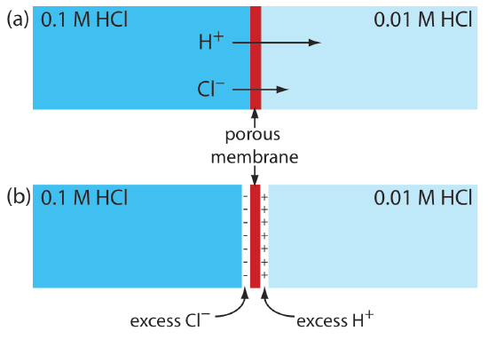
A junction potential develops at the interface between two ionic solutions if there is a difference in the concentration and the mobility of the ions. Consider, for example, a porous membrane that separates a solution of 0.1 M HCl from a solution of 0.01 M HCl (Figure \(\PageIndex{1}\)a). Because the concentration of HCl on the membrane’s left side is greater than that on the right side of the membrane, H⁺ and Cl^– will diffuse in the direction of the arrows. The mobility of H⁺, however, is greater than that for Cl^–, as shown by the difference in the lengths of their respective arrows. Because of this difference in mobility, the solution on the right side of the membrane develops an excess concentration of H⁺ and a positive charge (Figure \(\PageIndex{1}\)b). Simultaneously, the solution on the membrane’s left side develops a negative charge because there is an excess concentration of Cl^–. We call this difference in potential across the membrane a junction potential and represent it as E_j.

Figure \(\PageIndex{1}\). Origin of the junction potential between a solution of 0.1 M HCl and a solution of 0.01 M HCl.

The magnitude of a junction potential depends upon the difference in the concentration of ions on the two sides of the interface, and may be as large as 30–40 mV. For example, a junction potential of 33.09 mV has been measured at the interface between solutions of 0.1 M HCl and 0.1 M NaCl [Sawyer, D. T.; Roberts, J. L., Jr. Experimental Electrochemistry for Chemists, Wiley-Interscience: New York, 1974, p. 22]. A salt bridge’s junction potential is minimized by using a salt, such as KCl, for which the mobilities of the cation and anion are approximately equal. We also can minimize the junction potential by incorporating a high concentration of the salt in the salt bridge. For this reason salt bridges frequently are constructed using solutions that are saturated with KCl. Nevertheless, a small junction potential, generally of unknown magnitude, is always present.