16.1: Theory of Infrared Absorption Spectrometry

Understanding the IR Spectrum

Figure \(\PageIndex{1}\) shows the infrared spectrum for ethanol. Unlike a UV/Vis absorbance spectrum, the y-axis is displayed as percent transmittance (%T) instead of absorbance, reflecting the fact that IR is used more for qualitative purposes than for quantitative purposes, where Beer's law, which is a linear function of concentration (\(A = \epsilon b C\)) makes absorbance the more useful measurement. The x-axis for an IR spectrum usually is given in wavenumbers, \(\overline{\nu} = \lambda^{-1}\), with units of cm^–1. The peaks in an IR spectrum are inverted relative to absorbance spectrum; that is, they descend from a baseline of 100%T instead of rising from a baseline of zero absorbance.

Figure \(\PageIndex{1}\): Infrared (IR) spectrum for ethanol.

Dipole Changes

The energy of a photon of infrared radiation (see Figure \(\PageIndex{2}\)) is not sufficient to affect a change in the electronic energy levels of electrons, as in the UV/Vis atomic or molecular absorption or emission spectroscopies covered in Chapters 9, 10, and 12–15. Instead, infrared radiation is confined to changes in the vibrational energy states of molecules and molecular ions. To absorb an IR photon, the absorbing species must experience a change in its dipole moment, which allows the oscillation in the photon's electrical field to interact with an oscillation in charge within the absorbing species. If the two oscillations have the same frequency, then absorption is possible.

Note

Each vibrational energy state in Figure \(\PageIndex{2}\) also has a set of rotational energy states, which means that the peak for a particular change in vibrational energy levels may consist of a series of closely spaced lines, one for each of several changes in rotational energy. Because rotation is difficult for analytes that in liquid or solid forms, we usually see just a single, broad absorption line; for this reason, we will consider only vibrational transitions in this chapter.

Figure \(\PageIndex{2}\): Diagram showing two electronic energy levels, \(E_0\) and \(E_1\), each with five vibrational energy levels, \(\nu_0 - \nu_1\). Absorption of ultraviolet and visible radiation (shown by the blue arrows) leads to a change in the analyte's electronic energy levels and, possibly, a change in vibrational energy as well. A change in vibrational energy without a change in electronic energy levels occurs with the absorption of infrared radiation (shown by the red arrows).

Types of Molecular Vibrations

Although we tend to think of the atoms in a molecule as being rigidly fixed in space relative to each other, the individual atoms are in a constant state of motion: bond lengths increase and decrease by stretching and compressing, and bond angles change as the result of the bending of the bonds relative to each other. Figure \(\PageIndex{3}\) shows two different types of stretching (symmetric and asymmetric) and four different types of bending (in-plane rocking, in-plane scissoring, out-of-plane wagging, and out-of-plane twisting).

Figure \(\PageIndex{3}\): The six types of stretching and bending motions. For out-of-plane wagging and out-of-plane twisting, the plus sign \((+)\) indicates that the atom is moving toward the viewer and the minus sign (\(-\)) indicate that the atom is moving away from the viewer.

Even a simple molecule can have many vibrational modes that give rise to a peak in the IR spectrum, as is the case for ethanol (Figure \(\PageIndex{1}\)). The number of possible normal vibrational modes for a linear molecule is \(3N - 5\), where N is the number of atoms, and \(3N - 6\) for a non-linear molecule. Ethanol, for example, has \(3 \times 9 - 6 = 21\) possible vibrational modes. As we will see later in this section, some of these modes may not lead to a change in dipole moment, decreasing the number of peaks in the IR spectrum.

Note

Why does a non-linear molecule have \(3N - 6\) vibrational modes? Consider a molecule of methane, CH₄. Each of methane’s five atoms can move in one of three directions (x, y, and z) for a total of \(3 \times 5 = 15\) different ways in which the molecule’s atoms can move. A molecule can move in three ways: it can move from one place to another, which we call translational motion; it can rotate around an axis, which we call rotational motion; and its bonds can stretch and bend, which we call vibrational motion. Because the entire molecule can move in the x, y, and z directions, three of methane’s 15 different ways of moving are translational. In addition, the molecule can rotate about its x, y, and z axes, accounting for three additional forms of motion. This leaves \(15 - 3 - 3 = 9\) vibrational modes. A linear molecule, such as CO₂, has \(3N - 5\) vibrational modes because it can rotate around only two axes.

Mechanical Model of Stretching in a Diatomic Molecule

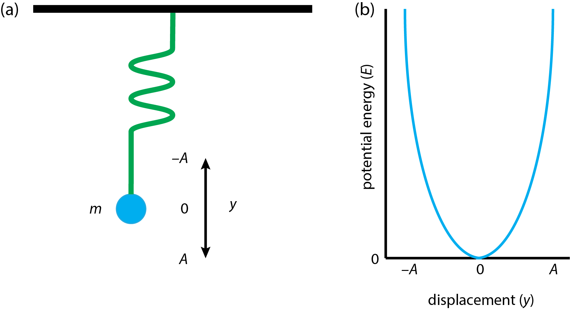
The simplest model system for the the stretching and compressing of a bond is a weight with a mass, m, attached to an ideal spring that hangs from the ceiling as shown in Figure \(\PageIndex{4}a\). If we pull on the mass and then release it, we initiate a simple oscillating harmonic motion that we can model using Hooke's law. If we displace the weight by a distance, y, then the force, F, that acts on the weight is

\[F = - k y \label{hookeslaw} \]

where \(k\) is the spring's force constant—a measure of the spring's springiness. The negative sign in Equation \ref{hookeslaw} indicates that this is the force needed to restore the spring to its original position; that is, the force is in the direction opposite to our action of pulling down on the weight.

Figure \(\PageIndex{4}\): The model for a simple harmonic oscillator is shown in (a) and its potential energy as a function of displacement is shown in (b).

Potential Energy of a Harmonic Oscillator

Let's take the potential energy, E, of the spring and weight as 0 when they are at rest (y = 0). If we pull down on the weight by a distance of \(dy\), then the change in the system's potential energy, \(dE\), must increase by the product of force and distance

\[dE = - F \times dy = - ky \times dy \label{PEchange} \]

Integrating Equation \ref{PEchange} from \(E = 0\) to \(E = E\) and from \(y = 0\) to \(y = y\)

\[\int_0^E dE = - k \int_0^y ydy \label{PEintegrals} \]

gives the energy as

\[E = \frac{1}{2} k y^2 \label{PE} \]

Figure \(\PageIndex{4}b\) shows the resulting potential energy curve, for which the maximum potential energy is \(\frac{1}{2}kA^2\) when the weight is at its maximum displacement. Note that the potential energy curve is a parabola.

Vibrational Frequency

The simple harmonic oscillator described above and shown in Figure \(\PageIndex{4}\) vibrates with a frequency, \(\nu_0\), given by the equation

\[\nu_0 = \frac{1}{2 \pi} \sqrt{\frac{k}{m}} \label{natfreq} \]

where \(k\) is the spring's force constant and \(m\) is the weight's mass. We can extend this to a spring that connects two weights to each other by substituting for the mass, \(m\), the system's reduced mass, \(\mu\)

\[\mu = \frac{m_1 \times m_2}{m_1 + m_2} \label{redmass} \]

where \(m_1\) and \(m_2\) are the masses of the two weights. Substituting Equation \ref{redmass} into Equation \ref{natfreq} gives

\[\nu_0 = \frac{1}{2 \pi} \sqrt{\frac{k}{\mu}} = \frac{1}{2 \pi} \sqrt{\frac{k(m_1 + m_2)}{m_1 \times m_2}} \label{natfreq2} \]

If we make the assumption that Equation \ref{natfreq2} applies to simple diatomic molecules, then we can estimate the bond's force constant, \(k\), by measuring its vibrational frequency.

Quantum Treatment of Vibrations

Equations \ref{PE}\ and \ref{natfreq2} are based on a classical mechanics treatment of the simple harmonic oscillator in which any displacement, and, thus, any energy is possible. Molecular vibrations, however, are quantized; thus

\[E = \left( v + \frac{1}{2} \right) \times h \times \frac{1}{2 \pi} \sqrt{\frac{k}{\mu}} = \left( v + \frac{1}{2} \right) h \nu_0 \label{quantizedE} \]

where \(v\) is the vibrational quantum number, which has allowed values of \(0, 1, 2, \dots\). The difference in energy, \(\Delta E\), between any two consecutive vibrational energy levels is \(h \nu_0\). As allowed transitions in quantum mechanics are limited to \(\Delta \nu = \pm 1\) and as the difference in energy is limited to \(\Delta E = h \nu_0\), any particular mode of vibration should give rise to a single peak.

Anharmonic Behavior

The ideal behavior described in the last section, in which each vibrational motion that produces a change in dipole moment results in a single peak, does not hold due to a variety of reasons, including the coulombic interactions between the atoms as they move toward and away from each other. One result of these non-ideal behaviors is that the value \(\Delta E\) does not remain constant for all values of the vibrational quantum number \(v\). For larger values of \(v\), the value of \(\Delta E\) becomes smaller and transitions where \(\Delta v = \pm 2\) or \(\Delta v = \pm 3\) become possible giving rise to what are called overtone lines at frequencies that are \(2 \times\) or \(3 \times\) that for \(\nu_0\).

Why Do We See More or Fewer Vibrational Peaks Than Expected?

Figure \(\PageIndex{5}\) shows the IR spectrum for carbon dioxide, CO₂, which consists of three clusters of peaks located at approximately 670 cm^–1, 2350 cm^–1, and 3700 cm^–1. As carbon dioxide is a linear molecule that consists of two carbon-oxygen double bonds (O=C=O), it has \(3 \times 3 - 5 = 9 - 5 = 4\) vibrational modes. So why do we see just three clusters of peaks?

Figure \(\PageIndex{5}\): IR spectrum for CO₂. The raw data is from NIST.

One of the requirements for the absorption of infrared radiation, is that the vibrational motion must result in a change in dipole moment. Figure \(\PageIndex{6}\) shows the four vibrational modes for CO₂. Of these four vibrational modes, the symmetric stretch does not result in a change in dipole moment. Although this appears to explain why we see just three clusters of peaks, a close examination of the two bending motions in Figure \(\PageIndex{6}\) should convince you that they are identical and, therefore, will appear as a single peak.

Figure \(\PageIndex{6}\): The four vibrational modes for CO₂. The symmetric stretch is not IR active as it does not involve a change in the molecules dipole moment. The asymmetric stretch occurs at 2349 cm^–1. The two bending motions are identical (or degenerate to each other) and appear at 667 cm^–1.

So what is the source of the cluster of peaks around 3700 cm^–1? Sometimes the absorption of a single photon excites two or more vibrational modes. In this case, the wavenumber for this absorption band is equivalent to the sum of the wavenumbers for the asymmetric stretch and the two degenerate bending modes (2349 + 667 = 3016 cm^–1, and 2349 + 667 + 667 = 3683 cm^–1). These are called combination bands.

Another source of additional peaks are overtone bands in which \(\Delta v = \pm 2\) or \(\Delta v = \pm 3\). Figure \(\PageIndex{7}\) shows the IR spectrum for carbonyl sulfide, OCS, which is analagous to CO₂ in which one of the oxygens is replaced with sulfur. The peak at 520 cm^–1 is for its two degenerate bending motions and is labeled \(\nu_2\). The asymmetric stretch at 2062 cm^–1 \((\nu_3)\) and the symmetric stretch at 859 cm^–1 \((\nu_1)\) are the other two fundamental absorption bands. The remaining peaks are overtones, such as the peak labeled \(2 \nu_2\) at 1040 cm^–1, or combination bands, such as the peak labeled \(\nu_3 + \nu_1\) at 2921 cm^–1. Many of the peaks appear as two peaks; this is the result of changes in rotational energy as well.

Figure \(\PageIndex{7}\): IR spectrum for OCS. The raw data is form NIST. The peak labeled as I (in red) is an impurity.