
9.2: Atomic Absorption Instrumentation
- Page ID
- 366343

\( \newcommand{\vecs}[1]{\overset { \scriptstyle \rightharpoonup} {\mathbf{#1}} } \)
\( \newcommand{\vecd}[1]{\overset{-\!-\!\rightharpoonup}{\vphantom{a}\smash {#1}}} \)
\( \newcommand{\id}{\mathrm{id}}\) \( \newcommand{\Span}{\mathrm{span}}\)
( \newcommand{\kernel}{\mathrm{null}\,}\) \( \newcommand{\range}{\mathrm{range}\,}\)
\( \newcommand{\RealPart}{\mathrm{Re}}\) \( \newcommand{\ImaginaryPart}{\mathrm{Im}}\)
\( \newcommand{\Argument}{\mathrm{Arg}}\) \( \newcommand{\norm}[1]{\| #1 \|}\)
\( \newcommand{\inner}[2]{\langle #1, #2 \rangle}\)
\( \newcommand{\Span}{\mathrm{span}}\)
\( \newcommand{\id}{\mathrm{id}}\)
\( \newcommand{\Span}{\mathrm{span}}\)
\( \newcommand{\kernel}{\mathrm{null}\,}\)
\( \newcommand{\range}{\mathrm{range}\,}\)
\( \newcommand{\RealPart}{\mathrm{Re}}\)
\( \newcommand{\ImaginaryPart}{\mathrm{Im}}\)
\( \newcommand{\Argument}{\mathrm{Arg}}\)
\( \newcommand{\norm}[1]{\| #1 \|}\)
\( \newcommand{\inner}[2]{\langle #1, #2 \rangle}\)
\( \newcommand{\Span}{\mathrm{span}}\) \( \newcommand{\AA}{\unicode[.8,0]{x212B}}\)
\( \newcommand{\vectorA}[1]{\vec{#1}} % arrow\)
\( \newcommand{\vectorAt}[1]{\vec{\text{#1}}} % arrow\)
\( \newcommand{\vectorB}[1]{\overset { \scriptstyle \rightharpoonup} {\mathbf{#1}} } \)
\( \newcommand{\vectorC}[1]{\textbf{#1}} \)
\( \newcommand{\vectorD}[1]{\overrightarrow{#1}} \)
\( \newcommand{\vectorDt}[1]{\overrightarrow{\text{#1}}} \)
\( \newcommand{\vectE}[1]{\overset{-\!-\!\rightharpoonup}{\vphantom{a}\smash{\mathbf {#1}}}} \)
\( \newcommand{\vecs}[1]{\overset { \scriptstyle \rightharpoonup} {\mathbf{#1}} } \)
\( \newcommand{\vecd}[1]{\overset{-\!-\!\rightharpoonup}{\vphantom{a}\smash {#1}}} \)
\(\newcommand{\avec}{\mathbf a}\) \(\newcommand{\bvec}{\mathbf b}\) \(\newcommand{\cvec}{\mathbf c}\) \(\newcommand{\dvec}{\mathbf d}\) \(\newcommand{\dtil}{\widetilde{\mathbf d}}\) \(\newcommand{\evec}{\mathbf e}\) \(\newcommand{\fvec}{\mathbf f}\) \(\newcommand{\nvec}{\mathbf n}\) \(\newcommand{\pvec}{\mathbf p}\) \(\newcommand{\qvec}{\mathbf q}\) \(\newcommand{\svec}{\mathbf s}\) \(\newcommand{\tvec}{\mathbf t}\) \(\newcommand{\uvec}{\mathbf u}\) \(\newcommand{\vvec}{\mathbf v}\) \(\newcommand{\wvec}{\mathbf w}\) \(\newcommand{\xvec}{\mathbf x}\) \(\newcommand{\yvec}{\mathbf y}\) \(\newcommand{\zvec}{\mathbf z}\) \(\newcommand{\rvec}{\mathbf r}\) \(\newcommand{\mvec}{\mathbf m}\) \(\newcommand{\zerovec}{\mathbf 0}\) \(\newcommand{\onevec}{\mathbf 1}\) \(\newcommand{\real}{\mathbb R}\) \(\newcommand{\twovec}[2]{\left[\begin{array}{r}#1 \\ #2 \end{array}\right]}\) \(\newcommand{\ctwovec}[2]{\left[\begin{array}{c}#1 \\ #2 \end{array}\right]}\) \(\newcommand{\threevec}[3]{\left[\begin{array}{r}#1 \\ #2 \\ #3 \end{array}\right]}\) \(\newcommand{\cthreevec}[3]{\left[\begin{array}{c}#1 \\ #2 \\ #3 \end{array}\right]}\) \(\newcommand{\fourvec}[4]{\left[\begin{array}{r}#1 \\ #2 \\ #3 \\ #4 \end{array}\right]}\) \(\newcommand{\cfourvec}[4]{\left[\begin{array}{c}#1 \\ #2 \\ #3 \\ #4 \end{array}\right]}\) \(\newcommand{\fivevec}[5]{\left[\begin{array}{r}#1 \\ #2 \\ #3 \\ #4 \\ #5 \\ \end{array}\right]}\) \(\newcommand{\cfivevec}[5]{\left[\begin{array}{c}#1 \\ #2 \\ #3 \\ #4 \\ #5 \\ \end{array}\right]}\) \(\newcommand{\mattwo}[4]{\left[\begin{array}{rr}#1 \amp #2 \\ #3 \amp #4 \\ \end{array}\right]}\) \(\newcommand{\laspan}[1]{\text{Span}\{#1\}}\) \(\newcommand{\bcal}{\cal B}\) \(\newcommand{\ccal}{\cal C}\) \(\newcommand{\scal}{\cal S}\) \(\newcommand{\wcal}{\cal W}\) \(\newcommand{\ecal}{\cal E}\) \(\newcommand{\coords}[2]{\left\{#1\right\}_{#2}}\) \(\newcommand{\gray}[1]{\color{gray}{#1}}\) \(\newcommand{\lgray}[1]{\color{lightgray}{#1}}\) \(\newcommand{\rank}{\operatorname{rank}}\) \(\newcommand{\row}{\text{Row}}\) \(\newcommand{\col}{\text{Col}}\) \(\renewcommand{\row}{\text{Row}}\) \(\newcommand{\nul}{\text{Nul}}\) \(\newcommand{\var}{\text{Var}}\) \(\newcommand{\corr}{\text{corr}}\) \(\newcommand{\len}[1]{\left|#1\right|}\) \(\newcommand{\bbar}{\overline{\bvec}}\) \(\newcommand{\bhat}{\widehat{\bvec}}\) \(\newcommand{\bperp}{\bvec^\perp}\) \(\newcommand{\xhat}{\widehat{\xvec}}\) \(\newcommand{\vhat}{\widehat{\vvec}}\) \(\newcommand{\uhat}{\widehat{\uvec}}\) \(\newcommand{\what}{\widehat{\wvec}}\) \(\newcommand{\Sighat}{\widehat{\Sigma}}\) \(\newcommand{\lt}{<}\) \(\newcommand{\gt}{>}\) \(\newcommand{\amp}{&}\) \(\definecolor{fillinmathshade}{gray}{0.9}\)Atomic absorption spectrophotometers use optical benches similar to those described earlier in Chapter 7, including a source of radiation, a method for introducing the sample (covered in the previous section), a means for isolating the wavelengths of interest, and a way to measure the amount of light absorbed or emitted.
Radiation Sources
Because atomic absorption lines are narrow, we need to use a line source instead of a continuum source to record atomic absorption spectra. Figure \(\PageIndex{1}\) will help us understand why this is necessary. As discussed in Chapter 7, a typical continuum source has an effective bandwidth on the order of 1 nm after passing through a monochromator. An atomic absorption line, as we learned in Chapter 8, has an effective line width on the order of 0.002 nm due to Doppler broadening and pressure broadening that takes place in a flame. If we pass the radiation from a continuum source through the flame, the incident power from the source, \(P_0\), and the power that reaches the detector, \(P_t\), are essentially identical, leading to an absorbance of zero. A line source, which operates a temperature that is lower than a flame, has a line width on the order of 0.001 nm. Passing this source radiation through the flame results in a measurable \(P_T\) and a measurable absorbance.

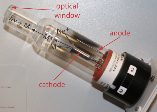
The source for atomic absorption is a hollow cathode lamp that consists of a cathode and anode enclosed within a glass tube filled with a low pressure of an inert gas, such as Ne or Ar (Figure \(\PageIndex{2}\)). Applying a potential across the electrodes ionizes the filler gas. The positively charged gas ions collide with the negatively charged cathode, sputtering atoms from the cathode’s surface. Some of the sputtered atoms are in the excited state and emit radiation characteristic of the metal(s) from which the cathode is manufactured. By fashioning the cathode from the metallic analyte, a hollow cathode lamp provides emission lines that correspond to the analyte’s absorption spectrum.
Each element in a hollow cathode lamp provides several atomic emission lines that we can use for atomic absorption. Usually the wavelength that provides the best sensitivity is the one we choose to use, although a less sensitive wavelength may be more appropriate for a sample that has higher concentration of analyte. For the Cr hollow cathode lamp in Table \(\PageIndex{1}\), the best sensitivity is obtained using a wavelength of 357.9 nm as this line requires the smallest concentration of analyte to achieve an absorbance of 0.20.
Another consideration is the emission line's intensity, \(P_0\). If several emission lines meet our requirements for sensitivity, we may wish to use the emission line with the largest relative P0 because there is less uncertainty in measuring P0 and PT. When analyzing a sample that is ≈10 mg Cr/L, for example, the first three wavelengths in Table \(\PageIndex{1}\) provide good sensitivity; the wavelengths of 425.4 nm and 429.0 nm, however, have a greater P0 and will provide less uncertainty in the measured absorbance.
The emission spectrum for a hollow cathode lamp includes, in addition to the analyte's emission lines, additional emission lines from impurities present in the metallic cathode and from the filler gas. These additional lines are a potential source of stray radiation that could result in an instrumental deviation from Beer’s law. The monochromator’s slit width is set as wide as possible to improve the throughput of radiation and narrow enough to eliminate these sources of stray radiation.
Optical Benches
Atomic absorption spectrometers are available using either a single-beam and a double-beam optical bench. Figure \(\PageIndex{3}\) shows a typical single-beam spectrometer, which consists of a hollow cathode lamp as a source, a flame, a grating monochromator, a detector (usually a photomultiplier tube), and a signal processor. Also included in this design is a chopper that periodically blocks light from the hollow cathode lamp from passing through the flame and reaching the detector. The purpose of the chopper is to provide a means for discriminating against the emission of light from the flame, which will otherwise contribute to the total amount of light that reaches the detector. As shown in Figure \(\PageIndex{3}\), when the chopper is closed, the only light reaching the detector is from the flame; emission from the flame and light from the lamp after it passes through the flame reach the detector when the chopper is open. The difference between the two signals gives the amount of light that reaches the detector after being absorbed by the sample. An alternative method that accomplishes the same thing is to modulate the amount of radiation emitted by the hollow cathode lamp.

Figure \(\PageIndex{4}\) shows the typical arrangement of a double-beam instrument for atomic absorption spectroscopy. In this design, the chopper alternates between two optical paths: one in which light from the hollow cathode lamp bypasses the flame and that measures the total emission of radiation from the flame and the lamp, and one that passes the hollow light from the hollow cathode lamp through the flame and that measures the emission of light from the flame and the amount of light from the hollow cathode lamp that is not absorbed by the sample. The difference between the two signals gives the amount of light that reaches the detector after being absorbed by the sample.
