8.1: Optical Atomic Spectra

Energy Level Diagrams

The energy of ultraviolet and visible electromagnetic radiation is sufficient to cause a change in an atom’s valence electron configuration. Sodium, for example, has a single valence electron in its 3s atomic orbital. As shown in Figure \(\PageIndex{1}\), unoccupied, higher energy atomic orbitals also exist. The valence shell energy level diagram in Figure \(\PageIndex{1}\) might strike you as odd because it shows the 3p orbitals split into two groups of slightly different energy (the two lines differ by just 0.6 nm). The cause of this splitting is a consequence of an electron's angular momentum and its spin. When these two are in the opposite direction, then the energy is slightly smaller than when the two are in the same direction. The effect is largest for p orbitals and sufficiently smaller for d and f orbitals that we do not bother to show the difference in their energies in this diagram.

Figure \(\PageIndex{1}\). Valence shell energy level diagram for sodium. The wavelengths (in nm) corresponding to several transitions are shown.

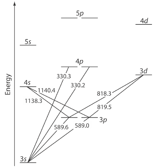
Absorption of a photon is accompanied by the excitation of an electron from a lower-energy atomic orbital to an atomic orbital of higher energy. Not all possible transitions between atomic orbitals are allowed. For sodium the only allowed transitions are those in which there is a change of ±1 in the orbital quantum number (l); thus transitions from \(s \rightarrow p\) orbitals are allowed, but transitions from \(s \rightarrow s\) and from \(s \rightarrow d\) orbitals are forbidden.

Atomic Absorption Spectra

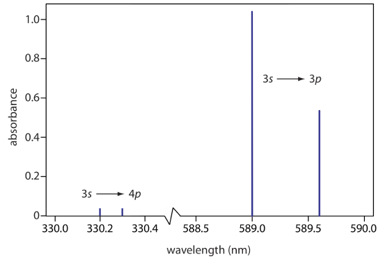
The atomic absorption spectrum for Na is shown in Figure \(\PageIndex{2}\), and is typical of that found for most atoms. The most obvious feature of this spectrum is that it consists of a small number of discrete absorption lines that correspond to transitions between the ground state (the 3s atomic orbital) and the 3p and the 4p atomic orbitals. Absorption from excited states, such as the \(3p \rightarrow 4s\) and the \(3p \rightarrow 3d\) transitions included in Figure \(\PageIndex{1}\), are too weak to detect. Because an excited state’s lifetime is short—an excited state atom typically returns to a lower energy state in 10^–7 to 10^–8 seconds—an atom in the exited state is likely to return to the ground state before it has an opportunity to absorb a photon.

Figure \(\PageIndex{2}\). Atomic absorption spectrum for sodium. Note that the scale on the x-axis includes a break.

Atomic Emission Spectra

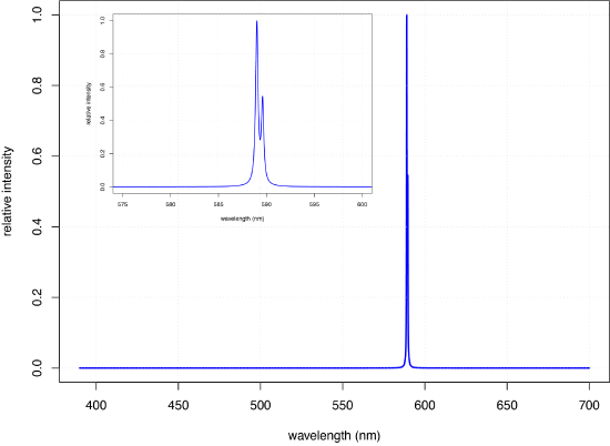
Atomic emission occurs when electrons in higher energy orbitals return to a lower energy state, releasing the excess energy as a photon. The ground state electron configuration for Na of \(1s^2 2s^2 2p^6 3s^1\) places a single electron in the \(3s\) valence shell. Introducing a solution of NaCl to a flame results in the formation of Na atoms (more on this in Chapter 9) and provides sufficient energy to promote the valence electron in the \(3s\) orbital to higher energy excited states, such as the \(3p\) orbitals identified in the energy level diagram for sodium in Figure \(\PageIndex{1}\). When an electron returns to its ground state, the excess energy is released as a photon. As seen in Figure \(\PageIndex{3}\), the emission spectrum for Na is dominated by the pair of lines with wavelengths of 589.0 and 589.6 nm.

Figure \(\PageIndex{3}\): Atomic emission spectrum for Na at a temperature of 3000 K. The inset shows that there are two closely spaced emission lines with wavelengths of 589.0 and 589.6 nm. The spectra were simulated using the R package atomicEmission.

Atomic Fluorescence Spectra

When an atom in an excited state emits a photon as a means of returning to a lower energy state, how we describe the process depends on the source of energy creating the excited state. When excitation is the result of thermal energy, as is the case for the spectrum in Figure \(\PageIndex{3}\), we call the process atomic emission spectroscopy. When excitation is the result of the absorption of a photon, we call the process atomic fluorescence spectroscopy. The absorption spectrum for Na in Figure \(\PageIndex{2}\) and its emission spectrum in Figure \(\PageIndex{2}\) shows that Na has both strong absorption and emission lines at 589.0 and 589.6 nm. If we use a source of light at 589.6 nm to move the 3s valence electron to a 3p excited state, we can then measure the emission of light at the same wavelength, making the measurement at 90° to avoid an interference from the original light source.

Fluorescence also may occur when an electron in an excited state first loses energy by a process other than the emission of a photon—we call this a radiationless transition—reaching a lower energy excited state from which it then emits a photon. For example, a ground state Na atom may first absorb a photon with a wavelength of 330.2 nm (a \(3s \rightarrow 4 p\) transition), which then loses energy through a radiationless transition to the 3p orbital where it then emits a photon to reach the 3s orbital.

Atomic Line Widths

Another feature of the atomic absorption spectrum in Figure \(\PageIndex{2}\) and the atomic emission spectrum in Figure \(\PageIndex{3}\) is the narrow width of the absorption and emission lines, which is a consequence of the fixed difference in energy between the ground state and the excited state, and the lack of vibrational and rotational energy levels. The width of an atomic absorption or emission line arises from several factors that we consider here.

Broadening Due to Uncertainty Principle

From the uncertainty principle, the product of the uncertainty of the frequency of light and the uncertainty in time must be greater than 1.

\[\Delta \nu \times \Delta t > 1 \nonumber \]

To determine the frequency with infinite precision, \(\Delta \nu = 0\), requires that the lifetime of an electron in a particular orbital must be infinitely large. While this may be essentially true for an electron in the ground state, it is not true for an electron in an excited state where the average lifetime—how long it takes before it returns to the ground state—may be on the order of \(10^{-7} \text{ to }10^{-8} \text{ s}\). For example, if \(\Delta t = 5 \times 10^{-8} \text{ s}\) for the emission of a photon with a wavelength of 500.0 nm, then

\[\Delta \nu = 2 \times 10^7 \text{ s}^{-1} \nonumber \]

To convert this an uncertainty in wavelength, \(\Delta \lambda\), we begin with the relationship

\[\nu = \frac{c}{\lambda} \nonumber \]

and take the derivative of \(\nu\) with respect to wavelength

\[d \nu = - \frac{c}{\lambda^2} d \lambda \nonumber \]

Rearranging to solve for the uncertainty in wavelength, and letting \(\Delta \nu\) and \(\Delta \lambda\) serve as estimates for \(d \nu\) and \(d \lambda\) leaves us with

\[ \left| \Delta \lambda \right| = \frac{\Delta \nu \times \lambda^2}{c} = \frac{(500.0 \times 10^{-9} \text{ m}^2) \times (2 \times 10^7 \text{s}^{-1})}{2.998 \times 10^8 \text{ m/s}} = 1.7 \times 10^{-14} \text{ m} \nonumber \]

or \(1.7 \times 10^{-5} \text{ nm}\). Natural line widths for atomic spectra are approximately 10^–5 nm.

Doppler Broadening and Pressure Broadening

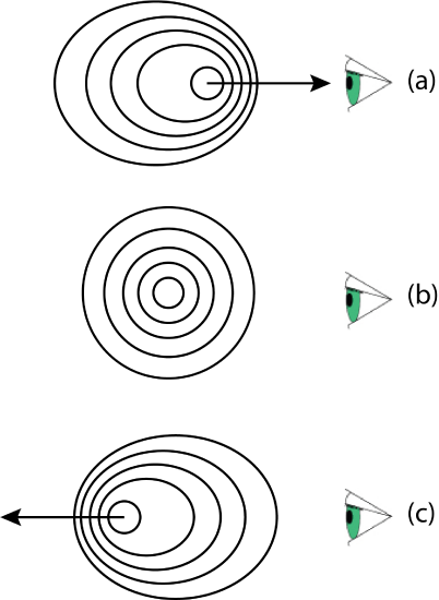
When an atom emits a photon, the frequency (and, thus, the wavelength) of the photon depends on whether the emitting atom is moving toward the detector or moving away from the detector. When the atom is moving toward the detector, as in Figure \(\PageIndex{4}a\), its emitted light reaches the detector at a greater frequency—a shorter wavelength—than when the light source is stationary, as in Figure \(\PageIndex{4}b\). An atom moving away from the detector, as in Figure \(\PageIndex{4}c\) emits light that reaches the detector with a smaller frequency and a longer wavelength.

Figure \(\PageIndex{4}\): Illustration showing the original of Doppler broadening. In (a) and (c) the atom is moving toward or away from the detector, respectively. In (b), the atom is stationary relative to the detector.

Atoms are in constant motion, which means that they also experience constant collisions, each of which results in a small change in the energy of an electron in the ground state or in an excited state, and a corresponding change in the wavelength emitted or absorbed. This effect is called pressure (or collisional) broadening. As is the case for Doppler broadening, pressure broadening increases with temperature. Together, Doppler broadening and pressure broadening result in an approximately 100-fold increase in line width, with line widths on the order of approximately 10^–3 nm.

Effect of Temperature on Atomic Spectra

As noted in the previous section, temperature contributes to the broadening of atomic absorption and atomic emission lines. Temperature also has an effect on the intensity of emission lines as it determines the relative population of an atom's various excited states. The Boltzmann distribution

\[\frac{N_i}{N_0} = \frac{P_i}{P_0} e^{-E_i/kT} \nonumber \]

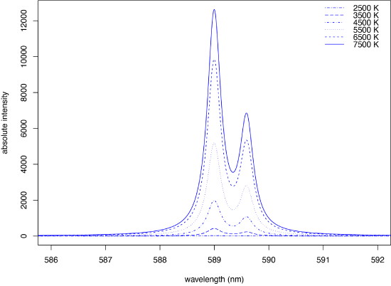
gives the relative number of atoms in a specific excited state, \(N_i\), relative to the number of atoms in the ground state, \(N_0\), as a function of the difference in their energies, \(E_i\), Boltzmann's constant, \(k\), the temperature in Kelvin, \(T\), and \(P_i\) and \(P_0\) are statistical factors that account for the number of equivalent energy states for the excited state and the ground state. Figure \(\PageIndex{5}\) shows how temperature affects the atomic emission spectrum for sodium's two intense emission lines at 589.0 and 589.6 nm for temperatures from 2500 K to 7500 K. Note that the emission at 2500 K is too small to appear using a y-axis scale of absolute intensities. A change in temperature from 5500 K to 4500 K reduces the emission intensity by 62%. As you might guess from this, a small change in temperature—perhaps as little as 10 K can result in a measurable decrease in emission intensity of a few percent.

Figure \(\PageIndex{5}\): Atomic emission spectra for Na as a function of temperature. The spectra were simulated using the R package atomicEmission.

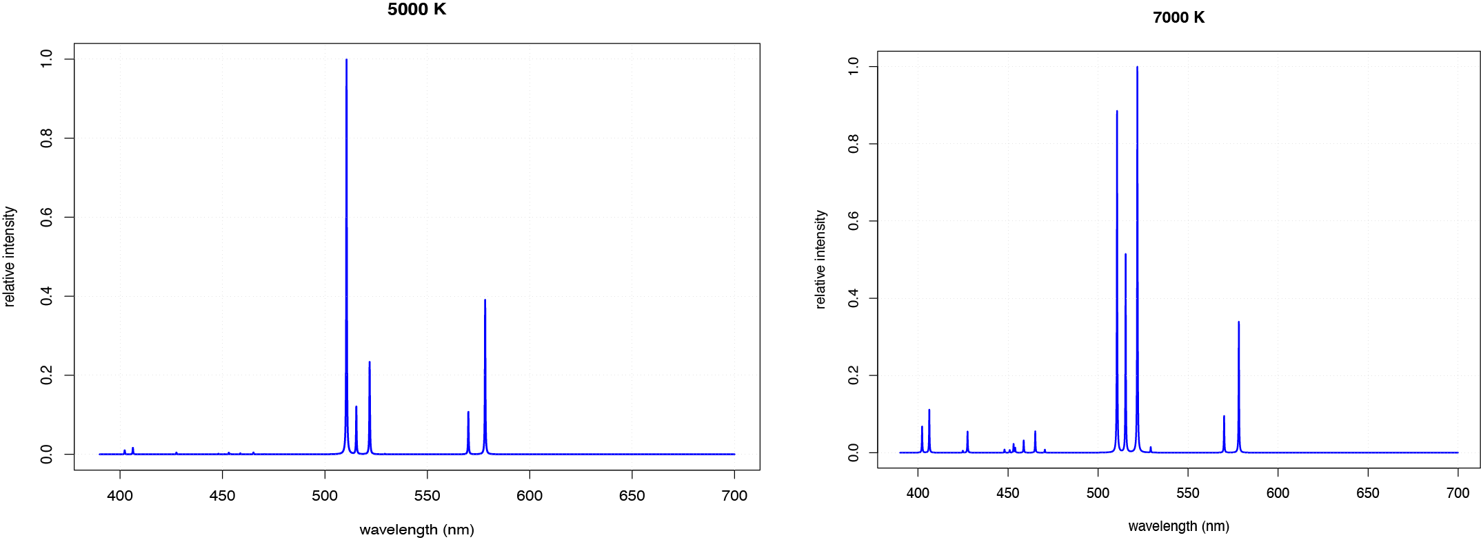
An increase in temperature may also change the relative emission intensity of different lines. Figure \(\PageIndex{6}\), for example, shows the atomic emission spectra for copper at 5000 K and 7000 K. At the higher temperature, the most intense emission line changes from 510.55 nm to 521.82 nm, and several additional peaks between 400 nm and 500 nm become more intense.

Figure \(\PageIndex{6}\): Atomic emission spectra for Cu at 5000 K and 7000 K. The spectra were simulated using the R package atomicEmission.

Band and Continuum Spectra

The atomic emission spectra for sodium in Figure \(\PageIndex{3}\) consists of discrete, narrow lines because they arise from the transition between the discrete, well-defined energy levels seen in Figure \(\PageIndex{1}\). Atomic emission from a flame also include contributions from two additional sources: the emission from molecular species that form in the flame and emission from the flame. A sample of water, for example, is likely to contain a variety of ions, such as Ca²⁺, that form molecular species, such as CaOH in the flame, and that emit photon over a much broader range of wavelengths than do atoms. The flame, itself, emits photons throughout the range of wavelengths used in UV/Vis atomic emission.