7.7: Fourier Transform Optical Spectroscopy

Thus far, the optical benches described in this chapter either use a single detector and a monochromator to pass a single wavelength of light to the detector, or use a multichannel array of detectors and a diffraction grating to disperse the light across the detectors. Both of these approaches have advantages and limitations. For the first of these designs, we can improve resolution by using a smaller slit width, although this comes with a decrease in the throughput of light that reaches the detector, which increases noise. Recording a complete spectrum requires scanning the monochromator; a slow scan rate can improve resolution by reducing the range of wavelengths reaching the detector per unit time, but at the expense of a longer analysis time, which is a problem if the composition of our samples changes with time. For the second of these designs, resolution is limited by the size of the array; for example, a spectral range of 190 nm to 800 nm and a photodiode array with 512 individual elements has a digital resolution of

\[\frac{800 - 190}{512} = 1.2 \text{ nm/diode} \nonumber \]

although the optical resolution—defined by the actual number of individual diodes over which a wavelength of light is dispersed—is greater and may vary with wavelength. Because a photodiode array allows for the simultaneous detection of radiation by each diode in the array, data acquisition is fast and a complete spectrum is acquired in approximately one second.

Interferometers

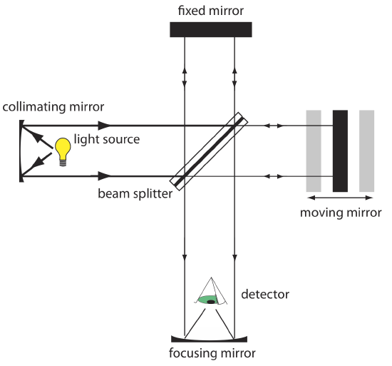
We can overcome the limitations described above if we can find a way to avoid dispersing the source radiation in time by scanning the monochromator, or dispersing the source radiation in space across an array of sensors. An interferometer, Figure \(\PageIndex{1}\), provides one way to accomplish this. Radiation from the source is collected by a collimating mirror and passed to a beam splitter where half of the radiation is directed toward a mirror set at a fixed distance from the beam splitter, and the other half of the radiation is passed through to a mirror that moves back and forth. The radiation from the two mirrors is recombined at the beam splitter and half of it is passed along to the detector.

Figure \(\PageIndex{1}\): Schematic diagram of an interferometer for use in optical spectroscopy. The distance of the fixed mirror and the moving mirror from the beam splitter is the same when the moving mirror is in the position shown in black.

Time Domain and Frequency Domain

When the radiation recombines at the beam splitter, constructive and destructive interference determines, for each wavelength, the intensity of light that reaches the detector. As the moving mirror changes position, the wavelength of light that experiences maximum constructive interference and maximum destructive interference also changes. The signal at the detector shows intensity as a function of the moving mirror’s position, expressed in units of distance or time. The result is called an interferogram or a time domain spectrum. The time domain spectrum is converted mathematically, by a process called a Fourier transform, to a spectrum (a frequency domain) that shows intensity as a function of the radiation’s frequency.

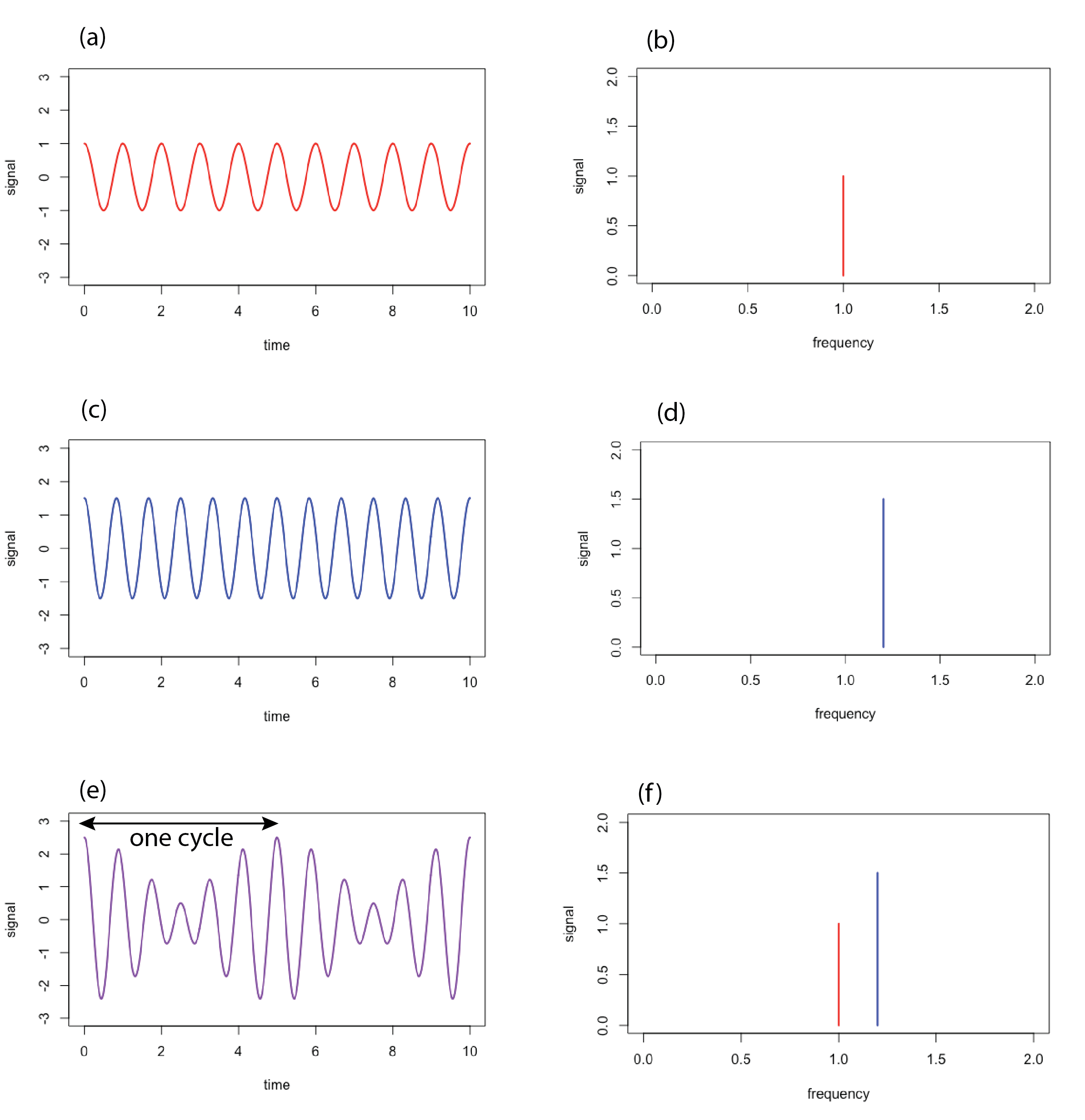
Figure \(\PageIndex{2}\) shows the relationship between the time domain spectrum and the frequency domain spectrum. The spectra in the first row show the relationship between (a) the time domain spectrum and (b) the corresponding frequency domain spectrum for a monochromatic source of radiation with a frequency, \(\nu_1\), of 1 and an amplitude, \(A_1\), of 1.0. In the time domain we see a simple cosine function with the general form

\[S = A_1 \times \cos{(2 \pi \nu_1 t)} \label{signal1} \]

where \(S\) is the signal and \(t\) is the time. The spectra in the second row show the same information for a second monochromatic source of radiation with a frequency, \(\nu_2\), of 1.2 and an amplitude, \(A_2\), of 1.5, which is given by the equation

\[S = A_2 \times \cos{(2 \pi \nu_2 t)} \label{signal2} \]

If we have a source that emits just these two frequencies of light, then the corresponding time domain and frequency domain spectra in the last row, where

\[S = A_1 \times \cos{(2 \pi \nu_1 t)} + A_2 \times \cos{(2 \pi \nu_2 t)} \label{signal3} \]

Although the time domain spectrum in panel (e) is more complex than those in panels (a) and (c), there is a clear repeating pattern, one cycle of which is shown by the arrow. Note that for each of these three examples, the time domain spectrum and the frequency domain spectrum encode the same information about the source radiation.

Figure \(\PageIndex{2}\): Time domain and frequency domain spectra for (a) and (b) a monochromatic source with a frequency of \(\nu_1\) and an amplitude of \(A_1\), for (c) and (d) a monochromatic source with a frequency of \(\nu_2\) and an amplitude of \(A_2\), and (e) and (f) a polychromatic source that consists of the two monochromatic sources.

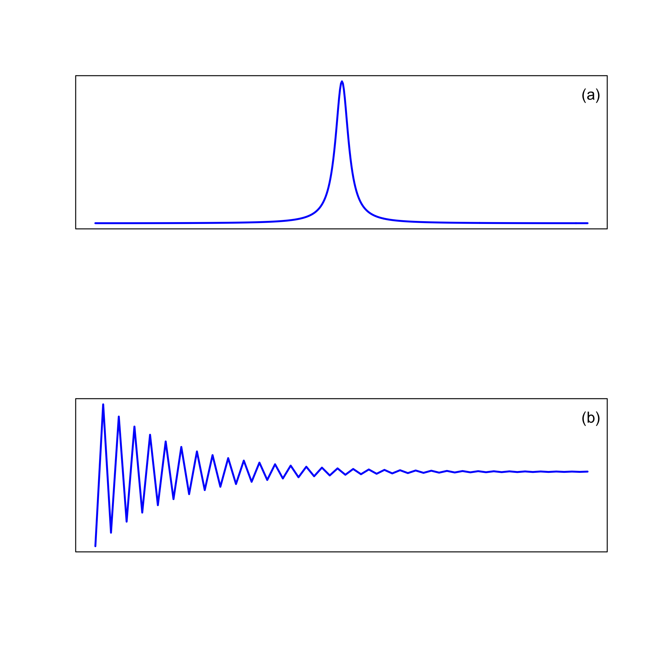
The two monochromatic signals in Figure \(\PageIndex{2}\) are line spectra with line widths that are essentially zero. But what if our signal has a measurable linewidth? We might consider such a signal to be the sum of a series of cosine functions, each with an amplitude and a frequency. Figure \(\PageIndex{3}a\) shows a frequency domain that contains a single peak with a finite width and Figure \(\PageIndex{3}b\) shows the corresponding time domain spectrum, which consists of an oscillating signal with an amplitude that decays over time. In general, Figure \(\PageIndex{2}\) and Figure \(\PageIndex{3}\) show that

• the further a peak in the frequency domain is from the origin, the greater its corresponding oscillation frequency in the time domain
• the broader a peak's width in the frequency domain, the faster its decay rate in the time domain
• the greater the area under a peak in the frequency domain, the higher its initial intensity in the time domain

Figure \(\PageIndex{3}\): The plot in (a) shows a frequency domain consisting of a single peak defined by its position along the x-axis, its width, and its area. The plot in (b) shows the corresponding time domain that consists of a single oscillating signal defined by its oscillation frequency, its initial intensity, and its decay rate.

The mathematical process of converting between the time domain and the frequency domain is called a Fourier transform. The details of the mathematics are sufficiently complex that calculations by hand are impractical.

Advantages of Fourier Transform Spectrometry

In comparison to a monochromator, an interferometer has several significant advantages. The first advantage, which is termed Jacquinot’s advantage, is the greater throughput of source radiation. Because an interferometer does not use slits and has fewer optical components from which radiation is scattered and lost, the throughput of radiation reaching the detector is \(80-200 \times\) greater than that for a monochromator. The result is less noise. A second advantage, which is called Fellgett’s advantage, is a savings in the time needed to obtain a spectrum. Because the detector monitors all frequencies simultaneously, a spectrum takes approximately one second to record, as compared to 10–15 minutes when using a scanning monochromator. A third advantage is that increased resolution is achieved by increasing the distance traveled by the moving mirror, which we can achieve without the need to decrease a scanniing monochromator's slit width or without increasing the size of an array detector.