
10.4: Using R to Clean Up Data
- Page ID
- 292497

\( \newcommand{\vecs}[1]{\overset { \scriptstyle \rightharpoonup} {\mathbf{#1}} } \)
\( \newcommand{\vecd}[1]{\overset{-\!-\!\rightharpoonup}{\vphantom{a}\smash {#1}}} \)
\( \newcommand{\id}{\mathrm{id}}\) \( \newcommand{\Span}{\mathrm{span}}\)
( \newcommand{\kernel}{\mathrm{null}\,}\) \( \newcommand{\range}{\mathrm{range}\,}\)
\( \newcommand{\RealPart}{\mathrm{Re}}\) \( \newcommand{\ImaginaryPart}{\mathrm{Im}}\)
\( \newcommand{\Argument}{\mathrm{Arg}}\) \( \newcommand{\norm}[1]{\| #1 \|}\)
\( \newcommand{\inner}[2]{\langle #1, #2 \rangle}\)
\( \newcommand{\Span}{\mathrm{span}}\)
\( \newcommand{\id}{\mathrm{id}}\)
\( \newcommand{\Span}{\mathrm{span}}\)
\( \newcommand{\kernel}{\mathrm{null}\,}\)
\( \newcommand{\range}{\mathrm{range}\,}\)
\( \newcommand{\RealPart}{\mathrm{Re}}\)
\( \newcommand{\ImaginaryPart}{\mathrm{Im}}\)
\( \newcommand{\Argument}{\mathrm{Arg}}\)
\( \newcommand{\norm}[1]{\| #1 \|}\)
\( \newcommand{\inner}[2]{\langle #1, #2 \rangle}\)
\( \newcommand{\Span}{\mathrm{span}}\) \( \newcommand{\AA}{\unicode[.8,0]{x212B}}\)
\( \newcommand{\vectorA}[1]{\vec{#1}} % arrow\)
\( \newcommand{\vectorAt}[1]{\vec{\text{#1}}} % arrow\)
\( \newcommand{\vectorB}[1]{\overset { \scriptstyle \rightharpoonup} {\mathbf{#1}} } \)
\( \newcommand{\vectorC}[1]{\textbf{#1}} \)
\( \newcommand{\vectorD}[1]{\overrightarrow{#1}} \)
\( \newcommand{\vectorDt}[1]{\overrightarrow{\text{#1}}} \)
\( \newcommand{\vectE}[1]{\overset{-\!-\!\rightharpoonup}{\vphantom{a}\smash{\mathbf {#1}}}} \)
\( \newcommand{\vecs}[1]{\overset { \scriptstyle \rightharpoonup} {\mathbf{#1}} } \)
\( \newcommand{\vecd}[1]{\overset{-\!-\!\rightharpoonup}{\vphantom{a}\smash {#1}}} \)
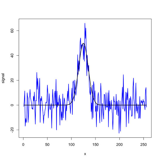
\(\newcommand{\avec}{\mathbf a}\) \(\newcommand{\bvec}{\mathbf b}\) \(\newcommand{\cvec}{\mathbf c}\) \(\newcommand{\dvec}{\mathbf d}\) \(\newcommand{\dtil}{\widetilde{\mathbf d}}\) \(\newcommand{\evec}{\mathbf e}\) \(\newcommand{\fvec}{\mathbf f}\) \(\newcommand{\nvec}{\mathbf n}\) \(\newcommand{\pvec}{\mathbf p}\) \(\newcommand{\qvec}{\mathbf q}\) \(\newcommand{\svec}{\mathbf s}\) \(\newcommand{\tvec}{\mathbf t}\) \(\newcommand{\uvec}{\mathbf u}\) \(\newcommand{\vvec}{\mathbf v}\) \(\newcommand{\wvec}{\mathbf w}\) \(\newcommand{\xvec}{\mathbf x}\) \(\newcommand{\yvec}{\mathbf y}\) \(\newcommand{\zvec}{\mathbf z}\) \(\newcommand{\rvec}{\mathbf r}\) \(\newcommand{\mvec}{\mathbf m}\) \(\newcommand{\zerovec}{\mathbf 0}\) \(\newcommand{\onevec}{\mathbf 1}\) \(\newcommand{\real}{\mathbb R}\) \(\newcommand{\twovec}[2]{\left[\begin{array}{r}#1 \\ #2 \end{array}\right]}\) \(\newcommand{\ctwovec}[2]{\left[\begin{array}{c}#1 \\ #2 \end{array}\right]}\) \(\newcommand{\threevec}[3]{\left[\begin{array}{r}#1 \\ #2 \\ #3 \end{array}\right]}\) \(\newcommand{\cthreevec}[3]{\left[\begin{array}{c}#1 \\ #2 \\ #3 \end{array}\right]}\) \(\newcommand{\fourvec}[4]{\left[\begin{array}{r}#1 \\ #2 \\ #3 \\ #4 \end{array}\right]}\) \(\newcommand{\cfourvec}[4]{\left[\begin{array}{c}#1 \\ #2 \\ #3 \\ #4 \end{array}\right]}\) \(\newcommand{\fivevec}[5]{\left[\begin{array}{r}#1 \\ #2 \\ #3 \\ #4 \\ #5 \\ \end{array}\right]}\) \(\newcommand{\cfivevec}[5]{\left[\begin{array}{c}#1 \\ #2 \\ #3 \\ #4 \\ #5 \\ \end{array}\right]}\) \(\newcommand{\mattwo}[4]{\left[\begin{array}{rr}#1 \amp #2 \\ #3 \amp #4 \\ \end{array}\right]}\) \(\newcommand{\laspan}[1]{\text{Span}\{#1\}}\) \(\newcommand{\bcal}{\cal B}\) \(\newcommand{\ccal}{\cal C}\) \(\newcommand{\scal}{\cal S}\) \(\newcommand{\wcal}{\cal W}\) \(\newcommand{\ecal}{\cal E}\) \(\newcommand{\coords}[2]{\left\{#1\right\}_{#2}}\) \(\newcommand{\gray}[1]{\color{gray}{#1}}\) \(\newcommand{\lgray}[1]{\color{lightgray}{#1}}\) \(\newcommand{\rank}{\operatorname{rank}}\) \(\newcommand{\row}{\text{Row}}\) \(\newcommand{\col}{\text{Col}}\) \(\renewcommand{\row}{\text{Row}}\) \(\newcommand{\nul}{\text{Nul}}\) \(\newcommand{\var}{\text{Var}}\) \(\newcommand{\corr}{\text{corr}}\) \(\newcommand{\len}[1]{\left|#1\right|}\) \(\newcommand{\bbar}{\overline{\bvec}}\) \(\newcommand{\bhat}{\widehat{\bvec}}\) \(\newcommand{\bperp}{\bvec^\perp}\) \(\newcommand{\xhat}{\widehat{\xvec}}\) \(\newcommand{\vhat}{\widehat{\vvec}}\) \(\newcommand{\uhat}{\widehat{\uvec}}\) \(\newcommand{\what}{\widehat{\wvec}}\) \(\newcommand{\Sighat}{\widehat{\Sigma}}\) \(\newcommand{\lt}{<}\) \(\newcommand{\gt}{>}\) \(\newcommand{\amp}{&}\) \(\definecolor{fillinmathshade}{gray}{0.9}\)R has two useful functions, filter() and fft(), that we can use to smooth or filter noise and to remove background signals. To explore their use, let's first create two sets of data that we can use as examples: a noisy signal and a pure signal superimposed on an exponential background. To create the noisy signal, we first create a vector of 256 values that defines the x-axis; although we will not specify a unit here, these could be times or frequencies. Next we use R's dnorm() function to generate a pure Gaussian signal with a mean of 125 and a standard deviation of 10, and R's rnorm() function to generate 256 points of random noise with a mean of zero and a standard deviation of 10. Finally, we add the pure signal and the noise to arrive at our noisy signal and then plot the noisy signal and overlay the pure signal.
x = seq(1,256,1)

gaus_signal = 1250 * dnorm(x, mean = 125, sd = 10)

noise = rnorm(256, mean = 0, sd = 10)

noisy_signal = gaus_signal + noise

plot(x = x, y = noisy_signal, type = "l", lwd = 2, col = "blue", xlab = "x", ylab = "signal")

lines(x = x, y = gaus_signal, lwd = 2)
To estimate the signal-to-noise ratio, we use the maximum of the pure signal and the standard deviation of the noisy signal as determined using 100 points divided evenly between the two ends.
s_to_n = max(gaus_signal)/sd(noisy_signal[c(1:50,201:250)])

s_to_n
[1] 5.14663
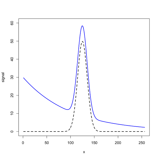
To create a signal superimposed on an exponential background, we use R's exp() function to generate 256 points for the background's signal, add that to our pure Gaussian signal, and plot the result.
exp_bkgd = 30*exp(-0.01 * x)

plot(x,exp_bkgd,type = "l")

signal_bkgd = gaus_signal + exp_bkgd

plot(x = x, y = signal_bkgd, type = "l", lwd = 2, col = "blue", xlab = "x", ylab = "signal", ylim = c(0,60))

lines(x = x, y = gaus_signal, lwd = 2, lty = 2)
Using R's filter() Function to Smooth Noise and Remove Background Signals
R's filter() function takes the general form
filter(x, filter)
where x is the object being filtered and filter is an object that contains the filter's coefficients. To create a seven-point moving average filter, we use the rep() function to create a vector that has seven identical values, each equal to 1/7.
mov_avg_7 = rep(1/7, 7)
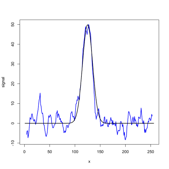
Applying this filter to our noisy signal returns the following result
noisy_signal_movavg = filter(noisy_signal, mov_avg_7)

plot(x = x, y = noisy_signal_movavg, type = "l", lwd = 2, col = "blue", xlab = "x", ylab = "signal")

lines(x = x, y = gaus_signal, lwd = 2)
with the signal-to-noise ratio improved to
s_to_n_movavg = max(gaus_signal)/sd(noisy_signal_movavg[c(1:50,200:250)], na.rm = TRUE)

s_to_n_movavg
[1] 11.29943
Note that we must add na.rm = TRUE to the sd() function because applying a seven-point moving average filter replaces the first three and the last three points with values of NA which we must tell the sd() function to ignore.
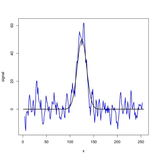
filter() function to apply a seven-point moving average filter to the noisy signal in Figure \(\PageIndex{1}\).To create a seven-point Savitzky-Golay smoothing filter, we create a vector to store the coefficients, obtaining the values from the original paper (Savitzky, A.; Golay, M. J. E. Anal Chem, 1964, 36, 1627-1639) and then apply it to our noisy signal, obtaining the results below.
sg_smooth_7 = c(-2,3,6,7,6,5,-2)/21

noisy_signal_sg = filter(noisy_signal, sg_smooth_7)

plot(x = x, y = noisy_signal_sg, type = "l", lwd = 2, col = "blue", xlab = "x", ylab = "signal")

lines(x = x, y = gaus_signal, lwd = 2)

s_to_n_movavg = max(gaus_signal)/sd(noisy_signal_sg[c(1:50,200:250)], na.rm = TRUE)

s_to_n_movavg
[1] 7.177931
filter() function to apply a seven-point Savitizky-Golay smooting filter to the noisy signal in Figure \(\PageIndex{1}\).To remove a background from a signal, we use the same approach, substituting a first-derivative (or higher order) Savitxky-Golay filter.
sg_fd_7 = c(22, -67, -58, 0, 58, 67, -22)/252

signal_bkgd_sg = filter(signal_bkgd, sg_fd_7)

plot(x = x, y = signal_bkgd_sg, type = "l", lwd = 2, col = "blue", xlab = "x", ylab = "signal")
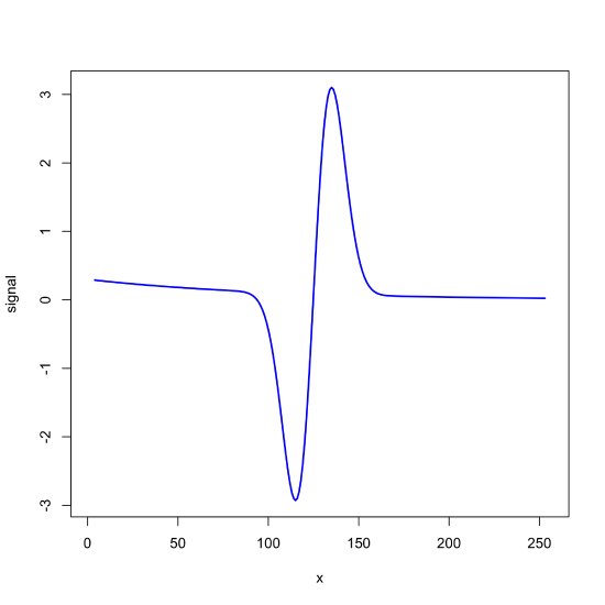
filter() function to apply a seven-point first-derivative Savitzky-Golay filter to the noisy signal in Figure \(\PageIndex{1}\).Using R's fft() Function for Fourier Filtering
To complete a Fourier transform in R we use the fft() function, which takes the form fft(z, inverse = FALSE) where z is the object that contains the values to which we wish to apply the Fourier transform and where setting inverse = TRUE allows for an inverse Fourier transform. Before we apply Fourier filtering to our noisy signal, let's first apply the fft() function to a vector that contains the integers 1 through 8. First we create a vector to hold our values and the apply the fft() function to the vector, obtaining the following results
test_vector = seq(1, 8, 1)

test_vector_ft = fft(test_vector)

test_vector_ft
[1] 36+0.000000i -4+9.656854i -4+4.000000i -4+1.656854i -4+0.000000i -4-1.656854i
[7] -4-4.000000i -4-9.656854i
Each of the eight results is a complex number with a real and an imaginary component. Note that the real component of the first value is 36, which is the sum of the elements in our test vector. Note, also, the symmetry in the remaining values where the second and eighth values, the third and seventh values, and the fourth and sixth values are identical except for a change in sign for the imaginary component.
Taking the inverse Fourier transform returns the original eight values (note that the imaginary terms are now zero), but each is eight times larger in value than in our original vector.
test_vector_ifft = fft(test_vector_ft, inverse = TRUE)

test_vector_ifft
[1] 8+0i 16-0i 24+0i 32+0i 40+0i 48+0i 56-0i 64+0i
To compensate for this, we divide by the length of our vector
test_vector_ifft = fft(test_vector_ft, inverse = TRUE)/length(test_vector)

test_vector_ifft
[1] 1+0i 2-0i 3+0i 4+0i 5+0i 6+0i 7-0i 8+0i
which returns our original vector.
With this background in place, let's use R to complete a Fourier filtering of our noisy signal. First, we complete the Fourier transform of the noisy signal and examine the values for the real component, using R's Re() function to extract them. Because of the symmetry noted above, we need only look at the first half of the real components (x = 1 to x = 128).
noisy_signal_ft = fft(noisy_signal)

plot(x = x[1:128], y = Re(noisy_signal_ft)[1:128], type = "l", col = "blue", xlab = "", ylab = "intensity", lwd = 2)
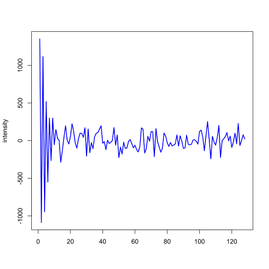
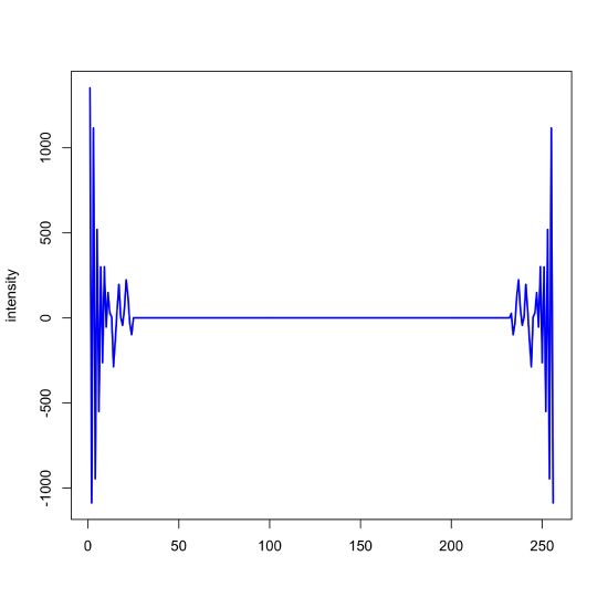
Next, we look for where the signal's magnitude has decayed to what appears to be random noise and set these values to zero. In this example, we retain the first 24 points (and the last 24 points; remember the symmetry noted above) and set both the real and the imaginary components to 0 + 0i.
noisy_signal_ft[25:232] = 0 + 0i

plot(x = x, y = Re(noisy_signal_ft), type = "l", col = "blue", xlab = "", ylab = "intensity", lwd = 2)
Finally, we take the inverse Fourier transform and display the resulting filtered signal and report the signal-to-noise ratio.
noisy_signal_ifft = fft(noisy_signal_ft, inverse = TRUE)/length(noisy_signal_ft)

plot(x = x, y = Re(noisy_signal_ifft), type = "l", col = "blue", xlab = "", ylab = "intensity", ylim = c(-20,60), lwd = 3)

lines(x = x,y = gaus_signal,lwd =2, col = "black")
s_to_n = 50/sd(Re(noisy_signal_ifft)[c(1:50,200:250)], na.rm = TRUE)

s_to_n
[1] 9.695329
