7.5: Using R for Significance Testing and Analysis of Variance

The base installation of R has functions for most of the significance tests covered in Chapter 7.2 - Chapter 7.4.

Using R to Compare Variances

The R function for comparing variances isvar.test()which takes the following form

var.test(x, y, ratio = 1, alternative = c("two.sided", "less", "greater"), conf.level = 0.95, ...)

where x and y are numeric vectors that contain the two samples, ratio is the expected ratio for the null hypothesis (which defaults to 1), alternative is a character string that states the alternative hypothesis (which defaults to two-sided or two-tailed), and a conf.level that gives the size of the confidence interval, which defaults to 0.95, or 95%, or \(\alpha = 0.05\). We can use this function to compare the variances of two samples, \(s_1^2\) vs \(s_2^2\), but not the variance of a sample and the variance for a population \(s^2\) vs \(\sigma^2\).

Let's use R on the data from Example 7.2.3, which considers two sets of United States pennies.

# create vectors to store the data

sample1 = c(3.080, 3.094, 3.107, 3.056, 3.112, 3.174, 3.198)

sample2 = c(3.052, 3.141, 3.083, 3.083, 3.048)

# run two-sided variance test with alpha = 0.05 and null hypothesis that variances are equal

var.test(x = sample1, y = sample2, ratio = 1, alternative = "two.sided", conf.level = 0.95)

The code above yields the following output

F test to compare two variances

data: sample1 and sample2

F = 1.8726, num df = 6, denom df = 4, p-value = 0.5661

alternative hypothesis: true ratio of variances is not equal to 1

95 percent confidence interval:

0.2036028 11.6609726

sample estimates: ratio of variances

1.872598

Two parts of this output lead us to retain the null hypothesis of equal variances. First, the reported p-value of 0.5661 is larger than our critical value for \(\alpha\) of 0.05, and second, the 95% confidence interval for the ratio of the variances, which runs from 0.204 to 11.7 includes the null hypothesis that it is 1.

R does not include a function for comparing \(s^2\) to \(\sigma^2\).

Using R to Compare Means

The R function for comparing means is t.test()and takes the following form

t.test(x, y = NULL, alternative = c("two.sided", "less", "greater"), mu = 0,

paired = FALSE, var.equal = FALSE, conf.level = 0.95, ...)

where x is a numeric vector that contains the data for one sample and y is an optional vector that contains data for a second sample, alternative is a character string that states the alternative hypothesis (which defaults to two-tailed), mu is either the population's expected mean or the expected difference in the means of the two samples, paired is a logical value that indicates whether the data is paired , var.equal is a logical value that indicates whether the variances for two samples are treated as equal or unequal (based on a prior var.test()), andconf.level gives the size of the confidence interval (which defaults to 0.95, or 95%, or \(\alpha = 0.05\)).

Using R to Compare \(\overline{X}\) to \(\mu\)

Let's use R on the data from Example 7.2.1, which considers the determination of the \(\% \text{Na}_2 \text{CO}_3\) in a standard sample that is known to be 98.76 % w/w \(\text{Na}_2 \text{CO}_3\).

# create vector to store the data

na2co3 = c(98.71, 98.59, 98.62, 98.44, 98.58)

# run a two-sided t-test, using mu to define the expected mean; because the default values

# for paired and var.equal are FALSE, we can omit them here

t.test(x = na2co3, alternative = "two.sided", mu = 98.76, conf.level = 0.95)

The code above yields the following output

One Sample t-test

data: na2co3

t = -3.9522, df = 4, p-value = 0.01679

alternative hypothesis: true mean is not equal to 98.76

95 percent confidence interval:

98.46717 98.70883

sample estimates:

mean of x

98.588

Two parts of this output lead us to reject the null hypothesis of equal variances. First, the reported p-value of 0.01679 is less than our critical value for \(\alpha\) of 0.05, and second, the 95% confidence interval for the experimental mean of 98.588, which runs from 98.467 to 98.709, does not includes the null hypothesis that it is 98.76.

Using R to Compare Means for Two Samples

When comparing the means for two samples, we have to be careful to consider whether the data is unpaired or paired, and for unpaired data we must determine whether we can pool the variances for the two samples.

Unpaired Data

Let's use R on the data from Example 7.2.4, which considers two sets of United States pennies. This data is unpaired and, as we showed earlier, there is no evidence to suggest that the variances of the two samples are different.

# create vectors to store the data

sample1 = c(3.080, 3.094, 3.107, 3.056, 3.112, 3.174, 3.198)

sample2 = c(3.052, 3.141, 3.083, 3.083, 3.048)

# run a two-sided t-test, setting mu to 0 as the null hypothesis is that the means are the same, and setting var.equal to TRUE

t.test(x = sample1, y = sample2, alternative = "two.sided", mu = 0, var.equal = TRUE, conf.level = 0.95)

The code above yields the following output

Two Sample t-test

data: sample1 and sample2

t = 1.3345, df = 10, p-value = 0.2116

alternative hypothesis: true difference in means is not equal to 0

95 percent confidence interval:

-0.02403040 0.09580182

sample estimates:

mean of x mean of y

3.117286 3.081400

Two parts of this output lead us to retain the null hypothesis of equal means. First, the reported p-value of 0.2116 is greater than our critical value for \(\alpha\) of 0.05, and second, the 95% confidence interval for the difference in the experimental means, which runs from -0.0240 to 0.0958, includes the null hypothesis that it is 0.

Paired Data

Let's use R on the data from Example 7.2.1, which compares two methods for determining the concentration of the antibiotic monensin in fermentation vats.

# create vectors to store the data

microbiological = c(129.5, 89.6, 76.6, 52.2, 110.8, 50.4, 72.4, 141.4, 75.0, 34.1, 60.3)

electrochemical = c(132.3, 91.0, 73.6, 58.2, 104.2, 49.9, 82.1, 154.1, 73.4, 38.1, 60.1)

# run a two-tailed t-test, setting mu to 0 as the null hypothesis is that the means are the same, and setting paired to TRUE

t.test(x = microbiological, y = electrochemical, alternative = "two.sided", mu = 0, paired = TRUE, conf.level = 0.95)

The code above yields the following output

Paired t-test

data: microbiological and electrochemical

t = -1.3225, df = 10, p-value = 0.2155

alternative hypothesis: true difference in means is not equal to 0

95 percent confidence interval:

-6.028684 1.537775

sample estimates:

mean of the differences

-2.245455

Two parts of this output lead us to retain the null hypothesis of equal means. First, the reported p-value of 0.2155 is greater than our critical value for \(\alpha\) of 0.05, and second, the 95% confidence interval for the difference in the experimental mean, which runs from -6.03 to 1.54, includes the null hypothesis that it is 0.

Using R to Detect Outliers

The base installation of R does not include tests for outliers, but the outliers package provided functions for Dixon's Q-test and Grubb's test. To install the package, use the following lines of code

install.packages("outliers")

library(outliers)

You only need to install the package once, but you must use library() to make the package available when you begin a new R session.

Dixon Q-test

The R function for Dixon's Q-test is dixon.test()and takes the following form

dixon.test(x, type, two.sided)

where x is a numeric vector with the data we are considering, type defines the specific value(s) that we are testing (we will use type = 10, which tests for a single outlier on either end of the ranked data), and two.sided, which indicates whether we use a one-tailed or two-tailed test (we will use two.sided = FALSE as we are interested in whether the smallest value is too small or the largest value is too large).

Let's use R on the data from Example 7.2.7, which considers the masses of a set of United States pennies.

penny = c(3.067, 2.514, 3.094, 3.049, 3.048, 3.109, 3.039, 3.079, 3.102)

dixon.test(x = penny, two.sided = FALSE, type = 10)

The code above yields the following output

Dixon test for outliers

data: penny Q = 0.88235, p-value < 2.2e-16

alternative hypothesis: lowest value 2.514 is an outlier

The reported p-value of less than \(2.2 \times 10^{-16}\) is less than our critical value for \(\alpha\) of 0.05, which suggests that the penny with a mass of 2.514 g is drawn from a different population than the other pennies.

Grubb's Test

The R function for the Grubb's test is grubbs.test()and takes the following form

gurbbs.test(x, type, two.sided)

where x is a numeric vector with the data we are considering, type defines the specific value(s) that we are testing (we will use type = 10, which tests for a single outlier on either end of the ranked data), and two.sided, which indicated whether we use a one-tailed or two-tailed test (we will use two.sided = FALSE as we are interested in whether the smallest value is too small or the largest value is too large).

Let's use R on the data from Example 7.2.7, which considers the masses of a set of United States pennies.

penny = c(3.067, 2.514, 3.094, 3.049, 3.048, 3.109, 3.039, 3.079, 3.102)

grubbs.test(x = penny, two.sided = FALSE, type = 10)

The code above yields the following output

Grubbs test for one outlier

data: penny

G = 2.64300, U = 0.01768, p-value = 9.69e-07

alternative hypothesis: lowest value 2.514 is an outlier

The reported p-value of \(9.69 \times 10^{-7}\) is less than our critical value for \(\alpha\) of 0.05, which suggests that the penny with a mass of 2.514 g is drawn from a different population than the other pennies.

Using R to Complete Non-Parametric Significance Tests

The R function for completing the Wilcoxson signed rank test and the Wilcoxson rank sum test is wilcox.test(), which takes the following form

wilcox.test(x, y = NULL, alternative = c("two.sided", "less", "greater"), mu = 0,

paired = FALSE, conf.level = 0.95, ...)

where x is a numeric vector that contains the data for one sample and y is an optional vector that contains data for a second sample, alternative is a character string that states the alternative hypothesis (which defaults to two-tailed), mu is either the population's expected mean or the expected difference in the means of the two samples, paired is a logical value that indicates whether the data is paired , andconf.level gives the size of the confidence interval (which defaults to 0.95, or 95%, or \(\alpha = 0.05\)).

Using R to Complete a Wilcoxson Signed Rank Test

Let's use R on the data from Example 7.3.1, which compares two methods for determining the concentration of the antibiotic monensin in fermentation vats.

# create vectors to store the data

microbiological = c(129.5, 89.6, 76.6, 52.2, 110.8, 50.4, 72.4, 141.4, 75.0, 34.1, 60.3)

electrochemical = c(132.3, 91.0, 73.6, 58.2, 104.2, 49.9, 82.1, 154.1, 73.4, 38.1, 60.1)

# run a two-tailed wilcoxson signed rank test, setting mu to 0 as the null hypothesis is that

# the means are the same and setting paired to TRUE

wilcox.test(x = microbiological, y = electrochemical, alternative = "two.sided", mu = 0, paired = TRUE, conf.level = 0.95)

The code above yields the following output

Wilcoxon signed rank test

data: microbiological and electrochemical

V = 22, p-value = 0.3652

alternative hypothesis: true location shift is not equal to 0

where the value V is the smaller of the two signed ranks. The reported p-value of 0.3652 is greater than our critical value for \(\alpha\) of 0.05, which means we do not have evidence to suggest that there is a difference between the mean values for the two methods.

Using R to Complete a Wilcoxson Rank Sum Test

Let's use R on the data from Example 7.3.2, which compares two methods for determining the amount of aspirin in tablets from two production lots.

# create vectors to store the data

lot1 = c(256, 248, 245, 244, 248, 261)

lot2= c(241, 258, 241, 256, 254)

# run a two-tailed wilcoxson signed rank test, setting mu to 0 as the null hypothesis is

# that the means are the same, and setting paired to TRUE

wilcox.test(x = lot1, y = lot2, alternative = "two.sided", mu = 0, paired = FALSE, conf.level = 0.95)

The code above yields the following output

Wilcoxon rank sum test with continuity correction

data: lot1 and lot2

W = 16.5, p-value = 0.8541

alternative hypothesis: true location shift is not equal to 0

Warning message:

In wilcox.test.default(x = lot1, y = lot2, alternative = "two.sided", : cannot compute exact p-value with ties

where the value W is the larger of the two ranked sums. The reported p-value of 0.8541 is greater than our critical value for \(\alpha\) of 0.05, which means we do not have evidence to suggest that there is a difference between the mean values for the two methods. Note: we can ignore the warning message here as our calculated value for p is very large relative to an \(\alpha\) of 0.05.

Using R to Complete an Analysis of Variance

Let's use the data in Example 7.3.1 to show how to complete an analysis of variance in R. First, we need to create individual numerical vectors for each treatment and then combine these vectors into a single numerical vector, which we will call recovery, that contains the results for each treatment.

a = c(101, 101, 104)

b = c(100, 98, 102)

c = c(90, 92, 94)

recovery = c(a, b, c)

We also need to create a vector of character strings that identifies the individual treatments for each element in the vector recovery.

treatment = c(rep("a", 3), rep("b", 3), rep("c", 3))

The R function for completing an analysis of variance is aov(), which takes the following form

aov(formula, ...)

where formula is a way of telling R to "explain this variable by using that variable." We will examine formulas in more detail in Chapter 8, but in this case the syntax is recovery ~ treatment , which means to model the recovery based on the treatment. In the code below, we assign the output of the aov() function to a variable so that we have access to the results of the analysis of variance

aov_output = aov(recovery ~ treatment)

through the summary() function

summary(aov_output)

Df Sum Sq Mean Sq F value Pr(>F)

treatment 2 168 84.00 22.91 0.00155 **

Residuals 6 22 3.67

--- Signif. codes: 0 ‘***’ 0.001 ‘**’ 0.01 ‘*’ 0.05 ‘.’ 0.1 ‘ ’ 1

Note that what we earlier called the between variance is identified here as the variance due to the treatments, and that we earlier called the within variance is identified her as the residual variance. As we saw in Example 7.3.1, the value for F_exp is significantly greater than the critical value for F at \(\alpha = 0.05\).

Having found evidence that there is a significant difference between the treatments, we can use R's TukeyHSD() function to identify the source(s) of that difference (HSD stands for Honest Significant Difference), which takes the general form

TukeyHSD(x, conf.level = 0.95, ...)

where x is an object that contains the results of an analysis of variance.

TukeyHSD(aov_output)

Tukey multiple comparisons of means

95% family-wise confidence level

Fit: aov(formula = recovery ~ treatment)

$treatment

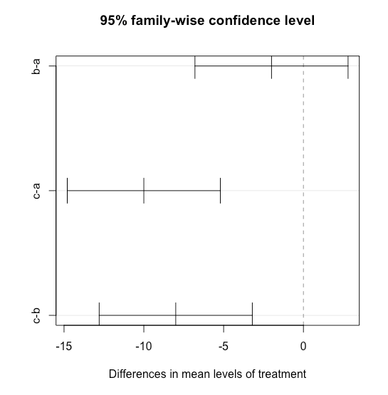
diff lwr upr p adj

b-a -2 -6.797161 2.797161 0.4554965

c-a -10 -14.797161 -5.202839 0.0016720

c-b -8 -12.797161 -3.202839 0.0052447

The table at the end of the output shows, for each pair of treatments, the difference in their mean values, the lower and the upper values for the confidence interval about the mean, and the value for \(\alpha\), which in R is listed as an adjusted p-value, for which we can reject the null hypothesis that the means are identical. In this case, we can see that the results for treatment C are significantly different from both treatments A and B.

We also can view the results of the TukeyHSD analysis visually by passing it to R's plot() function.

plot(TukeyHSD(aov_output))

Figure \(\PageIndex{1}\): Plot of the TukeyHSD results. The horizontal segments show the lower boundary and the upper boundary for the confidence interval about the difference between the mean values for each pair of treatments. The vertical dashed line shows a difference of zero. Those pairs of treatments with confidence intervals that do not include a difference of zero are significantly different from each other. Here we see evidence that treatment C is significantly different from both treatments A and B, but no evidence that treatments A and B are significantly different from each other.