
7.2: Significance Tests for Normal Distributions
- Page ID
- 221819

\( \newcommand{\vecs}[1]{\overset { \scriptstyle \rightharpoonup} {\mathbf{#1}} } \)
\( \newcommand{\vecd}[1]{\overset{-\!-\!\rightharpoonup}{\vphantom{a}\smash {#1}}} \)
\( \newcommand{\id}{\mathrm{id}}\) \( \newcommand{\Span}{\mathrm{span}}\)
( \newcommand{\kernel}{\mathrm{null}\,}\) \( \newcommand{\range}{\mathrm{range}\,}\)
\( \newcommand{\RealPart}{\mathrm{Re}}\) \( \newcommand{\ImaginaryPart}{\mathrm{Im}}\)
\( \newcommand{\Argument}{\mathrm{Arg}}\) \( \newcommand{\norm}[1]{\| #1 \|}\)
\( \newcommand{\inner}[2]{\langle #1, #2 \rangle}\)
\( \newcommand{\Span}{\mathrm{span}}\)
\( \newcommand{\id}{\mathrm{id}}\)
\( \newcommand{\Span}{\mathrm{span}}\)
\( \newcommand{\kernel}{\mathrm{null}\,}\)
\( \newcommand{\range}{\mathrm{range}\,}\)
\( \newcommand{\RealPart}{\mathrm{Re}}\)
\( \newcommand{\ImaginaryPart}{\mathrm{Im}}\)
\( \newcommand{\Argument}{\mathrm{Arg}}\)
\( \newcommand{\norm}[1]{\| #1 \|}\)
\( \newcommand{\inner}[2]{\langle #1, #2 \rangle}\)
\( \newcommand{\Span}{\mathrm{span}}\) \( \newcommand{\AA}{\unicode[.8,0]{x212B}}\)
\( \newcommand{\vectorA}[1]{\vec{#1}} % arrow\)
\( \newcommand{\vectorAt}[1]{\vec{\text{#1}}} % arrow\)
\( \newcommand{\vectorB}[1]{\overset { \scriptstyle \rightharpoonup} {\mathbf{#1}} } \)
\( \newcommand{\vectorC}[1]{\textbf{#1}} \)
\( \newcommand{\vectorD}[1]{\overrightarrow{#1}} \)
\( \newcommand{\vectorDt}[1]{\overrightarrow{\text{#1}}} \)
\( \newcommand{\vectE}[1]{\overset{-\!-\!\rightharpoonup}{\vphantom{a}\smash{\mathbf {#1}}}} \)
\( \newcommand{\vecs}[1]{\overset { \scriptstyle \rightharpoonup} {\mathbf{#1}} } \)
\( \newcommand{\vecd}[1]{\overset{-\!-\!\rightharpoonup}{\vphantom{a}\smash {#1}}} \)
\(\newcommand{\avec}{\mathbf a}\) \(\newcommand{\bvec}{\mathbf b}\) \(\newcommand{\cvec}{\mathbf c}\) \(\newcommand{\dvec}{\mathbf d}\) \(\newcommand{\dtil}{\widetilde{\mathbf d}}\) \(\newcommand{\evec}{\mathbf e}\) \(\newcommand{\fvec}{\mathbf f}\) \(\newcommand{\nvec}{\mathbf n}\) \(\newcommand{\pvec}{\mathbf p}\) \(\newcommand{\qvec}{\mathbf q}\) \(\newcommand{\svec}{\mathbf s}\) \(\newcommand{\tvec}{\mathbf t}\) \(\newcommand{\uvec}{\mathbf u}\) \(\newcommand{\vvec}{\mathbf v}\) \(\newcommand{\wvec}{\mathbf w}\) \(\newcommand{\xvec}{\mathbf x}\) \(\newcommand{\yvec}{\mathbf y}\) \(\newcommand{\zvec}{\mathbf z}\) \(\newcommand{\rvec}{\mathbf r}\) \(\newcommand{\mvec}{\mathbf m}\) \(\newcommand{\zerovec}{\mathbf 0}\) \(\newcommand{\onevec}{\mathbf 1}\) \(\newcommand{\real}{\mathbb R}\) \(\newcommand{\twovec}[2]{\left[\begin{array}{r}#1 \\ #2 \end{array}\right]}\) \(\newcommand{\ctwovec}[2]{\left[\begin{array}{c}#1 \\ #2 \end{array}\right]}\) \(\newcommand{\threevec}[3]{\left[\begin{array}{r}#1 \\ #2 \\ #3 \end{array}\right]}\) \(\newcommand{\cthreevec}[3]{\left[\begin{array}{c}#1 \\ #2 \\ #3 \end{array}\right]}\) \(\newcommand{\fourvec}[4]{\left[\begin{array}{r}#1 \\ #2 \\ #3 \\ #4 \end{array}\right]}\) \(\newcommand{\cfourvec}[4]{\left[\begin{array}{c}#1 \\ #2 \\ #3 \\ #4 \end{array}\right]}\) \(\newcommand{\fivevec}[5]{\left[\begin{array}{r}#1 \\ #2 \\ #3 \\ #4 \\ #5 \\ \end{array}\right]}\) \(\newcommand{\cfivevec}[5]{\left[\begin{array}{c}#1 \\ #2 \\ #3 \\ #4 \\ #5 \\ \end{array}\right]}\) \(\newcommand{\mattwo}[4]{\left[\begin{array}{rr}#1 \amp #2 \\ #3 \amp #4 \\ \end{array}\right]}\) \(\newcommand{\laspan}[1]{\text{Span}\{#1\}}\) \(\newcommand{\bcal}{\cal B}\) \(\newcommand{\ccal}{\cal C}\) \(\newcommand{\scal}{\cal S}\) \(\newcommand{\wcal}{\cal W}\) \(\newcommand{\ecal}{\cal E}\) \(\newcommand{\coords}[2]{\left\{#1\right\}_{#2}}\) \(\newcommand{\gray}[1]{\color{gray}{#1}}\) \(\newcommand{\lgray}[1]{\color{lightgray}{#1}}\) \(\newcommand{\rank}{\operatorname{rank}}\) \(\newcommand{\row}{\text{Row}}\) \(\newcommand{\col}{\text{Col}}\) \(\renewcommand{\row}{\text{Row}}\) \(\newcommand{\nul}{\text{Nul}}\) \(\newcommand{\var}{\text{Var}}\) \(\newcommand{\corr}{\text{corr}}\) \(\newcommand{\len}[1]{\left|#1\right|}\) \(\newcommand{\bbar}{\overline{\bvec}}\) \(\newcommand{\bhat}{\widehat{\bvec}}\) \(\newcommand{\bperp}{\bvec^\perp}\) \(\newcommand{\xhat}{\widehat{\xvec}}\) \(\newcommand{\vhat}{\widehat{\vvec}}\) \(\newcommand{\uhat}{\widehat{\uvec}}\) \(\newcommand{\what}{\widehat{\wvec}}\) \(\newcommand{\Sighat}{\widehat{\Sigma}}\) \(\newcommand{\lt}{<}\) \(\newcommand{\gt}{>}\) \(\newcommand{\amp}{&}\) \(\definecolor{fillinmathshade}{gray}{0.9}\)A normal distribution is the most common distribution for the data we collect. Because the area between any two limits of a normal distribution curve is well defined, it is straightforward to construct and evaluate significance tests.
You can review the properties of a normal distribution in Chapter 5 and Chapter 6.
Comparing \(\overline{X}\) to \(\mu\)
One way to validate a new analytical method is to analyze a sample that contains a known amount of analyte, \(\mu\). To judge the method’s accuracy we analyze several portions of the sample, determine the average amount of analyte in the sample, \(\overline{X}\), and use a significance test to compare \(\overline{X}\) to \(\mu\). The null hypothesis is that the difference between \(\overline{X}\) and \(\mu\) is explained by indeterminate errors that affect our determination of \(\overline{X}\). The alternative hypothesis is that the difference between \(\overline{X}\) and \(\mu\) is too large to be explained by indeterminate error.
\[H_0 \text{: } \overline{X} = \mu \nonumber\]
\[H_A \text{: } \overline{X} \neq \mu \nonumber\]
The test statistic is texp, which we substitute into the confidence interval for \(\mu\)
\[\mu = \overline{X} \pm \frac {t_\text{exp} s} {\sqrt{n}} \nonumber\]
Rearranging this equation and solving for \(t_\text{exp}\)
\[t_\text{exp} = \frac {|\mu - \overline{X}| \sqrt{n}} {s} \nonumber\]
gives the value for \(t_\text{exp}\) when \(\mu\) is at either the right edge or the left edge of the sample's confidence interval (Figure \(\PageIndex{1a}\)).
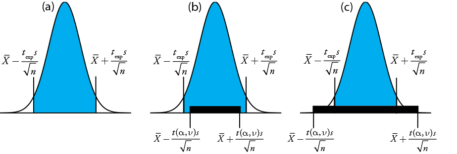
To determine if we should retain or reject the null hypothesis, we compare the value of texp to a critical value, \(t(\alpha, \nu)\), where \(\alpha\) is the confidence level and \(\nu\) is the degrees of freedom for the sample. The critical value \(t(\alpha, \nu)\) defines the largest confidence interval explained by indeterminate error. If \(t_\text{exp} > t(\alpha, \nu)\), then our sample’s confidence interval is greater than that explained by indeterminate errors (Figure \(\PageIndex{1}\)b). In this case, we reject the null hypothesis and accept the alternative hypothesis. If \(t_\text{exp} \leq t(\alpha, \nu)\), then our sample’s confidence interval is smaller than that explained by indeterminate error, and we retain the null hypothesis (Figure \(\PageIndex{1}\)c). Example \(\PageIndex{1}\) provides a typical application of this significance test, which is known as a t-test of \(\overline{X}\) to \(\mu\). You will find values for \(t(\alpha, \nu)\) in Appendix 2.
Before determining the amount of Na2CO3 in a sample, you decide to check your procedure by analyzing a standard sample that is 98.76% w/w Na2CO3. Five replicate determinations of the %w/w Na2CO3 in the standard gives the following results
\(98.71 \% \quad 98.59 \% \quad 98.62 \% \quad 98.44 \% \quad 98.58 \%\)
Using \(\alpha = 0.05\), is there any evidence that the analysis is giving inaccurate results?
Solution
The mean and standard deviation for the five trials are
\[\overline{X} = 98.59 \quad \quad \quad s = 0.0973 \nonumber\]
Because there is no reason to believe that the results for the standard must be larger or smaller than \(\mu\), a two-tailed t-test is appropriate. The null hypothesis and alternative hypothesis are
\[H_0 \text{: } \overline{X} = \mu \quad \quad \quad H_\text{A} \text{: } \overline{X} \neq \mu \nonumber\]
The test statistic, texp, is
\[t_\text{exp} = \frac {|\mu - \overline{X}|\sqrt{n}} {2} = \frac {|98.76 - 98.59| \sqrt{5}} {0.0973} = 3.91 \nonumber\]
The critical value for t(0.05, 4) from Appendix 2 is 2.78. Since texp is greater than t(0.05, 4), we reject the null hypothesis and accept the alternative hypothesis. At the 95% confidence level the difference between \(\overline{X}\) and \(\mu\) is too large to be explained by indeterminate sources of error, which suggests there is a determinate source of error that affects the analysis.
There is another way to interpret the result of this t-test. Knowing that texp is 3.91 and that there are 4 degrees of freedom, we use Appendix 2 to estimate the value of \(\alpha\) that corresponds to a t(\(\alpha\), 4) of 3.91. From Appendix 2, t(0.02, 4) is 3.75 and t(0.01, 4) is 4.60. Although we can reject the null hypothesis at the 98% confidence level, we cannot reject it at the 99% confidence level. For a discussion of the advantages of this approach, see J. A. C. Sterne and G. D. Smith “Sifting the evidence—what’s wrong with significance tests?” BMJ 2001, 322, 226–231.
Earlier we made the point that we must exercise caution when we interpret the result of a statistical analysis. We will keep returning to this point because it is an important one. Having determined that a result is inaccurate, as we did in Example \(\PageIndex{1}\), the next step is to identify and to correct the error. Before we expend time and money on this, however, we first should critically examine our data. For example, the smaller the value of s, the larger the value of texp. If the standard deviation for our analysis is unrealistically small, then the probability of a type 2 error increases. Including a few additional replicate analyses of the standard and reevaluating the t-test may strengthen our evidence for a determinate error, or it may show us that there is no evidence for a determinate error.
Comparing \(s^2\) to \(\sigma^2\)
If we analyze regularly a particular sample, we may be able to establish an expected variance, \(\sigma^2\), for the analysis. This often is the case, for example, in a clinical lab that analyzes hundreds of blood samples each day. A few replicate analyses of a single sample gives a sample variance, s2, whose value may or may not differ significantly from \(\sigma^2\).
We can use an F-test to evaluate whether a difference between s2 and \(\sigma^2\) is significant. The null hypothesis is \(H_0 \text{: } s^2 = \sigma^2\) and the alternative hypothesis is \(H_\text{A} \text{: } s^2 \neq \sigma^2\). The test statistic for evaluating the null hypothesis is Fexp, which is given as either
\[F_\text{exp} = \frac {s^2} {\sigma^2} \text{ if } s^2 > \sigma^2 \text{ or } F_\text{exp} = \frac {\sigma^2} {s^2} \text{ if } \sigma^2 > s^2 \nonumber\]
depending on whether s2 is larger or smaller than \(\sigma^2\). This way of defining Fexp ensures that its value is always greater than or equal to one.
If the null hypothesis is true, then Fexp should equal one; however, because of indeterminate errors, Fexp, usually is greater than one. A critical value, \(F(\alpha, \nu_\text{num}, \nu_\text{den})\), is the largest value of Fexp that we can attribute to indeterminate error given the specified significance level, \(\alpha\), and the degrees of freedom for the variance in the numerator, \(\nu_\text{num}\), and the variance in the denominator, \(\nu_\text{den}\). The degrees of freedom for s2 is n – 1, where n is the number of replicates used to determine the sample’s variance, and the degrees of freedom for \(\sigma^2\) is defined as infinity, \(\infty\). Critical values of F for \(\alpha = 0.05\) are listed in Appendix 3 for both one-tailed and two-tailed F-tests.
A manufacturer’s process for analyzing aspirin tablets has a known variance of 25. A sample of 10 aspirin tablets is selected and analyzed for the amount of aspirin, yielding the following results in mg aspirin/tablet.
\(254 \quad 249 \quad 252 \quad 252 \quad 249 \quad 249 \quad 250 \quad 247 \quad 251 \quad 252\)
Determine whether there is evidence of a significant difference between the sample’s variance and the expected variance at \(\alpha = 0.05\).
Solution
The variance for the sample of 10 tablets is 4.3. The null hypothesis and alternative hypotheses are
\[H_0 \text{: } s^2 = \sigma^2 \quad \quad \quad H_\text{A} \text{: } s^2 \neq \sigma^2 \nonumber\]
and the value for Fexp is
\[F_\text{exp} = \frac {\sigma^2} {s^2} = \frac {25} {4.3} = 5.8 \nonumber\]
The critical value for F(0.05, \(\infty\), 9) from Appendix 3 is 3.333. Since Fexp is greater than F(0.05, \(\infty\), 9), we reject the null hypothesis and accept the alternative hypothesis that there is a significant difference between the sample’s variance and the expected variance. One explanation for the difference might be that the aspirin tablets were not selected randomly.
Comparing Variances for Two Samples
We can extend the F-test to compare the variances for two samples, A and B, by rewriting our equation for Fexp as
\[F_\text{exp} = \frac {s_A^2} {s_B^2} \nonumber\]
defining A and B so that the value of Fexp is greater than or equal to 1.
The table below shows results for two experiments to determine the mass of a circulating U.S. penny. Determine whether there is a difference in the variances of these analyses at \(\alpha = 0.05\).
| First Experiment | Second Experiment | ||
|---|---|---|---|
| Penny | Mass (g) | Penny | Mass (g) |
| 1 | 3.080 | 1 | 3.052 |
| 2 | 3.094 | 2 | 3.141 |
| 3 | 3.107 | 3 | 3.083 |
| 4 | 3.056 | 4 | 3.083 |
| 5 | 3.112 | 5 | 3.048 |
| 6 | 3.174 | ||
| 7 | 3.198 | ||
Solution
The standard deviations for the two experiments are 0.051 for the first experiment (A) and 0.037 for the second experiment (B). The null and alternative hypotheses are
\[H_0 \text{: } s_A^2 = s_B^2 \quad \quad \quad H_\text{A} \text{: } s_A^2 \neq s_B^2 \nonumber\]
and the value of Fexp is
\[F_\text{exp} = \frac {s_A^2} {s_B^2} = \frac {(0.051)^2} {(0.037)^2} = \frac {0.00260} {0.00137} = 1.90 \nonumber\]
From Appendix 3 the critical value for F(0.05, 6, 4) is 9.197. Because Fexp < F(0.05, 6, 4), we retain the null hypothesis. There is no evidence at \(\alpha = 0.05\) to suggest that the difference in variances is significant.
Comparing Means for Two Samples
Three factors influence the result of an analysis: the method, the sample, and the analyst. We can study the influence of these factors by conducting experiments in which we change one factor while holding constant the other factors. For example, to compare two analytical methods we can have the same analyst apply each method to the same sample and then examine the resulting means. In a similar fashion, we can design experiments to compare two analysts or to compare two samples.
Before we consider the significance tests for comparing the means of two samples, we need to understand the difference between unpaired data and paired data. This is a critical distinction and learning to distinguish between these two types of data is important. Here are two simple examples that highlight the difference between unpaired data and paired data. In each example the goal is to compare two balances by weighing pennies.
- Example 1: We collect 10 pennies and weigh each penny on each balance. This is an example of paired data because we use the same 10 pennies to evaluate each balance.
- Example 2: We collect 10 pennies and divide them into two groups of five pennies each. We weigh the pennies in the first group on one balance and we weigh the second group of pennies on the other balance. Note that no penny is weighed on both balances. This is an example of unpaired data because we evaluate each balance using a different sample of pennies.
In both examples the samples of 10 pennies were drawn from the same population; the difference is how we sampled that population. We will learn why this distinction is important when we review the significance test for paired data; first, however, we present the significance test for unpaired data.
One simple test for determining whether data are paired or unpaired is to look at the size of each sample. If the samples are of different size, then the data must be unpaired. The converse is not true. If two samples are of equal size, they may be paired or unpaired.
Unpaired Data
Consider two analyses, A and B, with means of \(\overline{X}_A\) and \(\overline{X}_B\), and standard deviations of sA and sB. The confidence intervals for \(\mu_A\) and for \(\mu_B\) are
\[\mu_A = \overline{X}_A \pm \frac {t s_A} {\sqrt{n_A}} \nonumber\]
\[\mu_B = \overline{X}_B \pm \frac {t s_B} {\sqrt{n_B}} \nonumber\]
where nA and nB are the sample sizes for A and for B. Our null hypothesis, \(H_0 \text{: } \mu_A = \mu_B\), is that any difference between \(\mu_A\) and \(\mu_B\) is the result of indeterminate errors that affect the analyses. The alternative hypothesis, \(H_A \text{: } \mu_A \neq \mu_B\), is that the difference between \(\mu_A\)and \(\mu_B\) is too large to be explained by indeterminate error.
To derive an equation for texp, we assume that \(\mu_A\) equals \(\mu_B\), and combine the equations for the two confidence intervals
\[\overline{X}_A \pm \frac {t_\text{exp} s_A} {\sqrt{n_A}} = \overline{X}_B \pm \frac {t_\text{exp} s_B} {\sqrt{n_B}} \nonumber\]
Solving for \(|\overline{X}_A - \overline{X}_B|\) and using a propagation of uncertainty, gives
\[|\overline{X}_A - \overline{X}_B| = t_\text{exp} \times \sqrt{\frac {s_A^2} {n_A} + \frac {s_B^2} {n_B}} \nonumber\]
Finally, we solve for texp
\[t_\text{exp} = \frac {|\overline{X}_A - \overline{X}_B|} {\sqrt{\frac {s_A^2} {n_A} + \frac {s_B^2} {n_B}}} \nonumber\]
and compare it to a critical value, \(t(\alpha, \nu)\), where \(\alpha\) is the probability of a type 1 error, and \(\nu\) is the degrees of freedom.
Thus far our development of this t-test is similar to that for comparing \(\overline{X}\) to \(\mu\), and yet we do not have enough information to evaluate the t-test. Do you see the problem? With two independent sets of data it is unclear how many degrees of freedom we have.
Suppose that the variances \(s_A^2\) and \(s_B^2\) provide estimates of the same \(\sigma^2\). In this case we can replace \(s_A^2\) and \(s_B^2\) with a pooled variance, \(s_\text{pool}^2\), that is a better estimate for the variance. Thus, our equation for \(t_\text{exp}\) becomes
\[t_\text{exp} = \frac {|\overline{X}_A - \overline{X}_B|} {s_\text{pool} \times \sqrt{\frac {1} {n_A} + \frac {1} {n_B}}} = \frac {|\overline{X}_A - \overline{X}_B|} {s_\text{pool}} \times \sqrt{\frac {n_A n_B} {n_A + n_B}} \nonumber\]
where spool, the pooled standard deviation, is
\[s_\text{pool} = \sqrt{\frac {(n_A - 1) s_A^2 + (n_B - 1)s_B^2} {n_A + n_B - 2}} \nonumber\]
The denominator of this equation shows us that the degrees of freedom for a pooled standard deviation is \(n_A + n_B - 2\), which also is the degrees of freedom for the t-test. Note that we lose two degrees of freedom because the calculations for \(s_A^2\) and \(s_B^2\) require the prior calculation of \(\overline{X}_A\) amd \(\overline{X}_B\).
So how do you determine if it is okay to pool the variances? Use an F-test.
If \(s_A^2\) and \(s_B^2\) are significantly different, then we calculate texp using the following equation. In this case, we find the degrees of freedom using the following imposing equation.
\[\nu = \frac {\left( \frac {s_A^2} {n_A} + \frac {s_B^2} {n_B} \right)^2} {\frac {\left( \frac {s_A^2} {n_A} \right)^2} {n_A + 1} + \frac {\left( \frac {s_B^2} {n_B} \right)^2} {n_B + 1}} - 2 \nonumber\]
Because the degrees of freedom must be an integer, we round to the nearest integer the value of \(\nu\) obtained from this equation.
The equation above for the degrees of freedom is from Miller, J.C.; Miller, J.N. Statistics for Analytical Chemistry, 2nd Ed., Ellis-Horward: Chichester, UK, 1988. In the 6th Edition, the authors note that several different equations have been suggested for the number of degrees of freedom for t when sA and sB differ, reflecting the fact that the determination of degrees of freedom an approximation. An alternative equation—which is used by statistical software packages, such as R, Minitab, Excel—is
\[\nu = \frac {\left( \frac {s_A^2} {n_A} + \frac {s_B^2} {n_B} \right)^2} {\frac {\left( \frac {s_A^2} {n_A} \right)^2} {n_A - 1} + \frac {\left( \frac {s_B^2} {n_B} \right)^2} {n_B - 1}} = \frac {\left( \frac {s_A^2} {n_A} + \frac {s_B^2} {n_B} \right)^2} {\frac {s_A^4} {n_A^2(n_A - 1)} + \frac {s_B^4} {n_B^2(n_B - 1)}} \nonumber\]
For typical problems in analytical chemistry, the calculated degrees of freedom is reasonably insensitive to the choice of equation.
Regardless of whether how we calculate texp, we reject the null hypothesis if texp is greater than \(t(\alpha, \nu)\) and retain the null hypothesis if texp is less than or equal to \(t(\alpha, \nu)\).
Example \(\PageIndex{3}\) provides results for two experiments to determine the mass of a circulating U.S. penny. Determine whether there is a difference in the means of these analyses at \(\alpha = 0.05\).
Solution
First we use an F-test to determine whether we can pool the variances. We completed this analysis in Example \(\PageIndex{3}\), finding no evidence of a significant difference, which means we can pool the standard deviations, obtaining
\[s_\text{pool} = \sqrt{\frac {(7 - 1)(0.051)^2 + (5 - 1)(0.037)^2} {7 + 5 - 2}} = 0.0459 \nonumber\]
with 10 degrees of freedom. To compare the means we use the following null hypothesis and alternative hypotheses
\[H_0 \text{: } \mu_A = \mu_B \quad \quad \quad H_A \text{: } \mu_A \neq \mu_B \nonumber\]
Because we are using the pooled standard deviation, we calculate texp as
\[t_\text{exp} = \frac {|3.117 - 3.081|} {0.0459} \times \sqrt{\frac {7 \times 5} {7 + 5}} = 1.34 \nonumber\]
The critical value for t(0.05, 10), from Appendix 2, is 2.23. Because texp is less than t(0.05, 10) we retain the null hypothesis. For \(\alpha = 0.05\) we do not have evidence that the two sets of pennies are significantly different.
One method for determining the %w/w Na2CO3 in soda ash is to use an acid–base titration. When two analysts analyze the same sample of soda ash they obtain the results shown here.
Analyst A: \(86.82 \% \quad 87.04 \% \quad 86.93 \% \quad 87.01 \% \quad 86.20 \% \quad 87.00 \%\)
Analyst B: \(81.01 \% \quad 86.15 \% \quad 81.73 \% \quad 83.19 \% \quad 80.27 \% \quad 83.93 \% \quad\)
Determine whether the difference in the mean values is significant at \(\alpha = 0.05\).
Solution
We begin by reporting the mean and standard deviation for each analyst.
\[\overline{X}_A = 86.83\% \quad \quad s_A = 0.32\% \nonumber\]
\[\overline{X}_B = 82.71\% \quad \quad s_B = 2.16\% \nonumber\]
To determine whether we can use a pooled standard deviation, we first complete an F-test using the following null and alternative hypotheses.
\[H_0 \text{: } s_A^2 = s_B^2 \quad \quad \quad H_A \text{: } s_A^2 \neq s_B^2 \nonumber\]
Calculating Fexp, we obtain a value of
\[F_\text{exp} = \frac {(2.16)^2} {(0.32)^2} = 45.6 \nonumber\]
Because Fexp is larger than the critical value of 7.15 for F(0.05, 5, 5) from Appendix 3, we reject the null hypothesis and accept the alternative hypothesis that there is a significant difference between the variances; thus, we cannot calculate a pooled standard deviation.
To compare the means for the two analysts we use the following null and alternative hypotheses.
\[H_0 \text{: } \overline{X}_A = \overline{X}_B \quad \quad \quad H_A \text{: } \overline{X}_A \neq \overline{X}_B \nonumber\]
Because we cannot pool the standard deviations, we calculate texp as
\[t_\text{exp} = \frac {|86.83 - 82.71|} {\sqrt{\frac {(0.32)^2} {6} + \frac {(2.16)^2} {6}}} = 4.62 \nonumber\]
and calculate the degrees of freedom as
\[\nu = \frac {\left( \frac {(0.32)^2} {6} + \frac {(2.16)^2} {6} \right)^2} {\frac {\left( \frac {(0.32)^2} {6} \right)^2} {6 + 1} + \frac {\left( \frac {(2.16)^2} {6} \right)^2} {6 + 1}} - 2 = 5.3 \approx 5 \nonumber\]
From Appendix 2, the critical value for t(0.05, 5) is 2.57. Because texp is greater than t(0.05, 5) we reject the null hypothesis and accept the alternative hypothesis that the means for the two analysts are significantly different at \(\alpha = 0.05\).
Paired Data
Suppose we are evaluating a new method for monitoring blood glucose concentrations in patients. An important part of evaluating a new method is to compare it to an established method. What is the best way to gather data for this study? Because the variation in the blood glucose levels amongst patients is large we may be unable to detect a small, but significant difference between the methods if we use different patients to gather data for each method. Using paired data, in which the we analyze each patient’s blood using both methods, prevents a large variance within a population from adversely affecting a t-test of means.
Typical blood glucose levels for most non-diabetic individuals ranges between 80–120 mg/dL (4.4–6.7 mM), rising to as high as 140 mg/dL (7.8 mM) shortly after eating. Higher levels are common for individuals who are pre-diabetic or diabetic.
When we use paired data we first calculate the individual differences, di, between each sample's paired resykts. Using these individual differences, we then calculate the average difference, \(\overline{d}\), and the standard deviation of the differences, sd. The null hypothesis, \(H_0 \text{: } d = 0\), is that there is no difference between the two samples, and the alternative hypothesis, \(H_A \text{: } d \neq 0\), is that the difference between the two samples is significant.
The test statistic, texp, is derived from a confidence interval around \(\overline{d}\)
\[t_\text{exp} = \frac {|\overline{d}| \sqrt{n}} {s_d} \nonumber\]
where n is the number of paired samples. As is true for other forms of the t-test, we compare texp to \(t(\alpha, \nu)\), where the degrees of freedom, \(\nu\), is n – 1. If texp is greater than \(t(\alpha, \nu)\), then we reject the null hypothesis and accept the alternative hypothesis. We retain the null hypothesis if texp is less than or equal to t(a, o). This is known as a paired t-test.
Marecek et. al. developed a new electrochemical method for the rapid determination of the concentration of the antibiotic monensin in fermentation vats [Marecek, V.; Janchenova, H.; Brezina, M.; Betti, M. Anal. Chim. Acta 1991, 244, 15–19]. The standard method for the analysis is a test for microbiological activity, which is both difficult to complete and time-consuming. Samples were collected from the fermentation vats at various times during production and analyzed for the concentration of monensin using both methods. The results, in parts per thousand (ppt), are reported in the following table.
| Sample | Microbiological | Electrochemical |
|---|---|---|
| 1 | 129.5 | 132.3 |
| 2 | 89.6 | 91.0 |
| 3 | 76.6 | 73.6 |
| 4 | 52.2 | 58.2 |
| 5 | 110.8 | 104.2 |
| 6 | 50.4 | 49.9 |
| 7 | 72.4 | 82.1 |
| 8 | 141.4 | 154.1 |
| 9 | 75.0 | 73.4 |
| 10 | 34.1 | 38.1 |
| 11 | 60.3 | 60.1 |
Is there a significant difference between the methods at \(\alpha = 0.05\)?
Solution
Acquiring samples over an extended period of time introduces a substantial time-dependent change in the concentration of monensin. Because the variation in concentration between samples is so large, we use a paired t-test with the following null and alternative hypotheses.
\[H_0 \text{: } \overline{d} = 0 \quad \quad \quad H_A \text{: } \overline{d} \neq 0 \nonumber\]
Defining the difference between the methods as
\[d_i = (X_\text{elect})_i - (X_\text{micro})_i \nonumber\]
we calculate the difference for each sample.
| sample | 1 | 2 | 3 | 4 | 5 | 6 | 7 | 8 | 9 | 10 | 11 |
| \(d_i\) | 2.8 | 1.4 | –3.0 | 6.0 | –6.6 | –0.5 | 9.7 | 12.7 | –1.6 | 4.0 | –0.2 |
The mean and the standard deviation for the differences are, respectively, 2.25 ppt and 5.63 ppt. The value of texp is
\[t_\text{exp} = \frac {|2.25| \sqrt{11}} {5.63} = 1.33 \nonumber\]
which is smaller than the critical value of 2.23 for t(0.05, 10) from Appendix 2. We retain the null hypothesis and find no evidence for a significant difference in the methods at \(\alpha = 0.05\).
One important requirement for a paired t-test is that the determinate and the indeterminate errors that affect the analysis must be independent of the analyte’s concentration. If this is not the case, then a sample with an unusually high concentration of analyte will have an unusually large di. Including this sample in the calculation of \(\overline{d}\) and sd gives a biased estimate for the expected mean and standard deviation. This rarely is a problem for samples that span a limited range of analyte concentrations, such as those in Example \(\PageIndex{4}\) or Exercise \(\PageIndex{6}\). When paired data span a wide range of concentrations, however, the magnitude of the determinate and indeterminate sources of error may not be independent of the analyte’s concentration; when true, a paired t-test may give misleading results because the paired data with the largest absolute determinate and indeterminate errors will dominate \(\overline{d}\). In this situation a regression analysis, which is the subject of the next chapter, is more appropriate method for comparing the data.
The importance of distinguishing between paired and unpaired data is worth examining more closely. The following is data from some work I completed with a colleague in which we were looking at concentration of Zn in Lake Erie at the air-water interface and the sediment-water interface.
| sample site | ppm Zn at air-water interface | ppm Zn at the sediment-water interface |
| 1 | 0.430 | 0.415 |
| 2 | 0.266 | 0.238 |
| 3 | 0.457 | 0.390 |
| 4 | 0.531 | 0.410 |
| 5 | 0.707 | 0.605 |
| 6 | 0.716 | 0.609 |
The mean and the standard deviation for the ppm Zn at the air-water interface are 0.5178 ppm and 0.01732 ppm, and the mean and the standard deviation for the ppm Zn at the sediment-water interface are 0.4445 ppm and 0.1418 ppm. We can use these values to draw normal distributions for both by letting the means and the standard deviations for the samples, \(\overline{X}\) and \(s\), serve as estimates for the means and the standard deviations for the population, \(\mu\) and \(\sigma\). As we see in the following figure
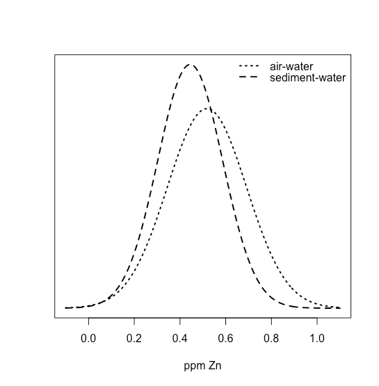
the two distributions overlap strongly, suggesting that a t-test of their means is not likely to find evidence of a difference. And yet, we also see that for each site, the concentration of Zn at the sediment-water interface is less than that at the air-water interface. In this case, the difference between the concentration of Zn at individual sites is sufficiently large that it masks our ability to see the difference between the two interfaces.
If we take the differences between the air-water and sediment-water interfaces, we have values of 0.015, 0.028, 0.067, 0.121, 0.102, and 0.107 ppm Zn, with a mean of 0.07333 ppm Zn and a standard deviation of 0.04410 ppm Zn. Superimposing all three normal distributions
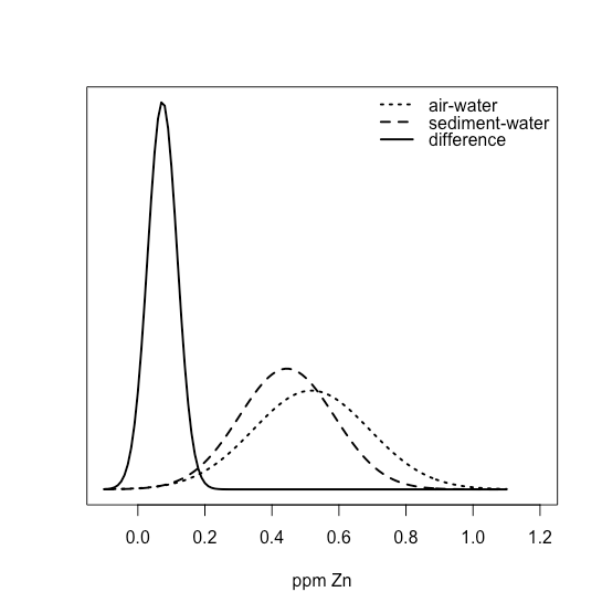
shows clearly that most of the normal distribution for the differences lies above zero, suggesting that a t-test might show evidence that the difference is significant.
Outliers
In chapter 7.1 we examined a data set consisting of the masses of 100 circulating United States penny. Table \(\PageIndex{1}\) provides one more data set. Do you notice anything unusual in this data? Of the 100 pennies included in the earlier table, no penny has a mass of less than 3 g. In this table, however, the mass of one penny is less than 3 g. We might ask whether this penny’s mass is so different from the other pennies that it is in error.
| 3.067 | 2.514 | 3.094 |
| 3.049 | 3.048 | 3.109 |
| 3.039 | 3.079 | 3.102 |
A measurement that is not consistent with other measurements is called an outlier. An outlier might exist for many reasons: the outlier might belong to a different population
Is this a Canadian penny?
or the outlier might be a contaminated or an otherwise altered sample
Is the penny damaged or unusually dirty?
or the outlier may result from an error in the analysis
Did we forget to tare the balance?
Regardless of its source, the presence of an outlier compromises any meaningful analysis of our data. There are many significance tests that we can use to identify a potential outlier, three of which we present here.
Dixon's Q-Test
One of the most common significance tests for identifying an outlier is Dixon’s Q-test. The null hypothesis is that there are no outliers, and the alternative hypothesis is that there is an outlier. The Q-test compares the gap between the suspected outlier and its nearest numerical neighbor to the range of the entire data set (Figure \(\PageIndex{2}\)).
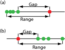
The test statistic, Qexp, is
\[Q_\text{exp} = \frac {\text{gap}} {\text{range}} = \frac {|\text{outlier's value} - \text{nearest value}|} {\text{largest value} - \text{smallest value}} \nonumber\]
This equation is appropriate for evaluating a single outlier. Other forms of Dixon’s Q-test allow its extension to detecting multiple outliers [Rorabacher, D. B. Anal. Chem. 1991, 63, 139–146].
The value of Qexp is compared to a critical value, \(Q(\alpha, n)\), where \(\alpha\) is the probability that we will reject a valid data point (a type 1 error) and n is the total number of data points. To protect against rejecting a valid data point, usually we apply the more conservative two-tailed Q-test, even though the possible outlier is the smallest or the largest value in the data set. If Qexp is greater than \(Q(\alpha, n)\), then we reject the null hypothesis and may exclude the outlier. We retain the possible outlier when Qexp is less than or equal to \(Q(\alpha, n)\). Table \(\PageIndex{2}\) provides values for \(Q(\alpha, n)\) for a data set that has 3–10 values. A more extensive table is in Appendix 4. Values for \(Q(\alpha, n)\) assume an underlying normal distribution.
| n | Q(0.05, n) |
|---|---|
| 3 | 0.970 |
| 4 | 0.829 |
| 5 | 0.710 |
| 6 | 0.625 |
| 7 | 0.568 |
| 8 | 0.526 |
| 9 | 0.493 |
| 10 | 0.466 |
Grubb's Test
Although Dixon’s Q-test is a common method for evaluating outliers, it is no longer favored by the International Standards Organization (ISO), which recommends the Grubb’s test. There are several versions of Grubb’s test depending on the number of potential outliers. Here we will consider the case where there is a single suspected outlier.
For details on this recommendation, see International Standards ISO Guide 5752-2 “Accuracy (trueness and precision) of measurement methods and results–Part 2: basic methods for the determination of repeatability and reproducibility of a standard measurement method,” 1994.
The test statistic for Grubb’s test, Gexp, is the distance between the sample’s mean, \(\overline{X}\), and the potential outlier, \(X_\text{out}\), in terms of the sample’s standard deviation, s.
\[G_\text{exp} = \frac {|X_\text{out} - \overline{X}|} {s} \nonumber\]
We compare the value of Gexp to a critical value \(G(\alpha, n)\), where \(\alpha\) is the probability that we will reject a valid data point and n is the number of data points in the sample. If Gexp is greater than \(G(\alpha, n)\), then we may reject the data point as an outlier, otherwise we retain the data point as part of the sample. Table \(\PageIndex{3}\) provides values for G(0.05, n) for a sample containing 3–10 values. A more extensive table is in Appendix 5. Values for \(G(\alpha, n)\) assume an underlying normal distribution.
| n | G(0.05, n) |
|---|---|
| 3 | 1.115 |
| 4 | 1.481 |
| 5 | 1.715 |
| 6 | 1.887 |
| 7 | 2.020 |
| 8 | 2.126 |
| 9 | 2.215 |
| 10 | 2.290 |
Chauvenet's Criterion
Our final method for identifying an outlier is Chauvenet’s criterion. Unlike Dixon’s Q-Test and Grubb’s test, you can apply this method to any distribution as long as you know how to calculate the probability for a particular outcome. Chauvenet’s criterion states that we can reject a data point if the probability of obtaining the data point’s value is less than \((2n^{-1})\), where n is the size of the sample. For example, if n = 10, a result with a probability of less than \((2 \times 10)^{-1}\), or 0.05, is considered an outlier.
To calculate a potential outlier’s probability we first calculate its standardized deviation, z
\[z = \frac {|X_\text{out} - \overline{X}|} {s} \nonumber\]
where \(X_\text{out}\) is the potential outlier, \(\overline{X}\) is the sample’s mean and s is the sample’s standard deviation. Note that this equation is identical to the equation for Gexp in the Grubb’s test. For a normal distribution, we can find the probability of obtaining a value of z using the probability table in Appendix 1.
Table \(\PageIndex{1}\) contains the masses for nine circulating United States pennies. One entry, 2.514 g, appears to be an outlier. Determine if this penny is an outlier using a Q-test, Grubb’s test, and Chauvenet’s criterion. For the Q-test and Grubb’s test, let \(\alpha = 0.05\).
Solution
For the Q-test the value for \(Q_\text{exp}\) is
\[Q_\text{exp} = \frac {|2.514 - 3.039|} {3.109 - 2.514} = 0.882 \nonumber\]
From Table \(\PageIndex{2}\), the critical value for Q(0.05, 9) is 0.493. Because Qexp is greater than Q(0.05, 9), we can assume the penny with a mass of 2.514 g likely is an outlier.
For Grubb’s test we first need the mean and the standard deviation, which are 3.011 g and 0.188 g, respectively. The value for Gexp is
\[G_\text{exp} = \frac {|2.514 - 3.011|} {0.188} = 2.64 \nonumber\]
Using Table \(\PageIndex{3}\), we find that the critical value for G(0.05, 9) is 2.215. Because Gexp is greater than G(0.05, 9), we can assume that the penny with a mass of 2.514 g likely is an outlier.
For Chauvenet’s criterion, the critical probability is \((2 \times 9)^{-1}\), or 0.0556. The value of z is the same as Gexp, or 2.64. Using Appendix 1, the probability for z = 2.64 is 0.00415. Because the probability of obtaining a mass of 0.2514 g is less than the critical probability, we can assume the penny with a mass of 2.514 g likely is an outlier.
You should exercise caution when using a significance test for outliers because there is a chance you will reject a valid result. In addition, you should avoid rejecting an outlier if it leads to a precision that is much better than expected based on a propagation of uncertainty. Given these concerns it is not surprising that some statisticians caution against the removal of outliers [Deming, W. E. Statistical Analysis of Data; Wiley: New York, 1943 (republished by Dover: New York, 1961); p. 171].
You also can adopt a more stringent requirement for rejecting data. When using the Grubb’s test, for example, the ISO 5752 guidelines suggest retaining a value if the probability for rejecting it is greater than \(\alpha = 0.05\), and flagging a value as a “straggler” if the probability for rejecting it is between \(\alpha = 0.05\) and \(\alpha = 0.01\). A “straggler” is retained unless there is compelling reason for its rejection. The guidelines recommend using \(\alpha = 0.01\) as the minimum criterion for rejecting a possible outlier.
On the other hand, testing for outliers can provide useful information if we try to understand the source of the suspected outlier. For example, the outlier in Table \(\PageIndex{1}\) represents a significant change in the mass of a penny (an approximately 17% decrease in mass), which is the result of a change in the composition of the U.S. penny. In 1982 the composition of a U.S. penny changed from a brass alloy that was 95% w/w Cu and 5% w/w Zn (with a nominal mass of 3.1 g), to a pure zinc core covered with copper (with a nominal mass of 2.5 g) [Richardson, T. H. J. Chem. Educ. 1991, 68, 310–311]. The pennies in Table \(\PageIndex{1}\), therefore, were drawn from different populations.