1.5: ICP-AES Analysis of Nanoparticles

What is ICP-AES?

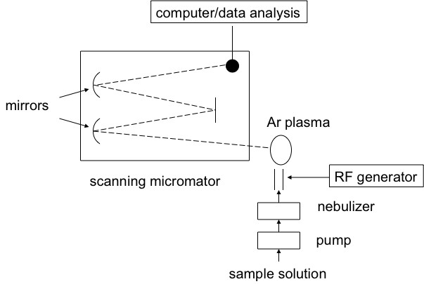
Inductively coupled plasma atomic emission spectroscopy (ICP-AES) is a spectral method used to determine very precisely the elemental composition of samples; it can also be used to quantify the elemental concentration with the sample. ICP-AES uses high-energy plasma from an inert gas like argon to burn analytes very rapidly. The color that is emitted from the analyte is indicative of the elements present, and the intensity of the spectral signal is indicative of the concentration of the elements that is present. A schematic view of a typical experimental set-up is shown here.

Figure \(\PageIndex{1}\): Schematic representation of an ICP-AES set-up.

How does ICP-AES work?

ICP-AES works by the emission of photons from analytes that are brought to an excited state by the use of high-energy plasma. The plasma source is induced when passing argon gas through an alternating electric field that is created by an inductively couple coil. When the analyte is excited the electrons try to dissipate the induced energy moving to a ground state of lower energy, in doing this they emit the excess energy in the form of light. The wavelength of light emitted depends on the energy gap between the excited energy level and the ground state. This is specific to the element based on the number of electrons the element has and electron orbital’s are filled. In this way the wavelength of light can be used to determine what elements are present by detection of the light at specific wavelengths.

As a simple example consider the situation when placing a piece of copper wire into the flame of a candle. The flame turns green due to the emission of excited electrons within the copper metal, as the electrons try to dissipate the energy incurred from the flame, they move to a more stable state emitting energy in the form of light. The energy gap between the excited state to the ground state (\(ΔE\) dictates the color of the light or wavelength of the light, Equation \ref{eq:DeltaE}, where \(h\) is Plank's constant (6.626×10^-34 m²kg/s), and \(\nu\) is the frequency of the emitted light.

\[ \Delta E = h \nu \label{eq:DeltaE} \]

The wavelength of light is indicative of the element present. If another metal is placed in the flame such as iron a different color flame will be emitted because the electronic structure of iron is different from that of copper. This is a very simple analogy for what is happening in ICP-AES and how it is used to determine what elements are present. By detecting the wavelength of light that is emitted from the analyte one can deduce what elements are be present.

Naturally if there is a lot of the material present then there will be an accumulative effect making the intensity of the signal large. However, if there were very little materials present the signal would be low. By this rationale one can create a calibration curve from analyte solutions of known concentrations, whereby the intensity of the signal changes as a function of the concentration of the material that is present. When measuring the intensity from a sample of unknown concentration the intensity from this sample can be compared to that from the calibration curve, so this can be used to determine the concentration of the analytes within the sample.

ICP-AES of Nanoparticles to Determine Elemental Composition

As with any sample being studied by ICP-AES nanoparticles need to be digested so that all the atoms can be vaporized in the plasma equally. If a metal containing nanoparticle were not digested using a strong acid to bring the metals atoms into solution, the form of the particle could hinder some of the material being vaporized. The analyte would not be detected even though it is present in the sample and this would give an erroneous result. Nanoparticles are often covered with a protective layer of organic ligands and this must be removed also. Further to this the solvent used for the nanoparticles may also be an organic solution and this should be removed as it too will not be miscible in the aqueous medium.

Several organic solvents have low vapor pressures so it is relatively easy to remove the solvent by heating the samples, removing the solvent by evaporation. To remove the organic ligands that are present on the nanoparticle, choric acid can be used. This is a very strong acid and can break down the organic ligands readily. To digest the particles and get the metal into solution concentrated nitric acid is often used.

A typical protocol may use 0.5 mL of concentrated nanoparticle solution and digest this with 9.5 mL of concentrated nitric acid over the period of a few days. After which 0.5 mL of the digested solution is placed in 9.5 mL of nanopure water. The reason why nanopure water is used is because DI water or regular water will have some amount of metals ions present and these will be detected by the ICP-AES measurement and will lead to figures that are not truly representative of the analyte concentration alone. This is especially pertinent when there is a very a low concentration of metal analyte to be detected, and is even more a problem when the metal to be detected is commonly found in water such as iron. Once the nanopure water and digested solution are prepared then the sample is ready for analysis.

Another point to consider when doing ICP-AES on nanoparticles to determine chemical compositions, includes the potential for wavelength overlap. The energy that is released in the form of light is unique to each element, but elements that are very similar in atomic structure will have emission wavelengths that are very similar to one another. Consider the example of iron and cobalt, these are both transition metals and sit right beside each other on the periodic table. Iron has an emission wavelength at 238.204 nm and cobalt has an emission wavelength at 238.892 nm. So if you were to try determine the amount of each element in an alloy of the two you would have to select another wavelength that would be unique to that element, and not have any wavelength overlap to other analytes in solution. For this case of iron and cobalt it would be wiser to use a wavelength for iron detection of 259.940 nm and a wavelength detection of 228.616 nm. Bearing this in mind a good rule of thumb is to try use the wavelength of the analyte that affords the best detection primarily. But if this value leads to a possible wavelength overlap of within 15 nm wavelength with another analyte in the solution then another choice should be made of the detection wavelength to prevent wavelength overlap from occurring.

Some people have also used the ICP-AES technique to determine the size of nanoparticles. The signal that is detected is determined by the amount of the material that is present in solution. If very dilute solutions of nanoparticles are being analyzed, particles are being analyzed one at a time, i.e., there will be one nanoparticle per droplet in the nebulizer. The signal intensity would then differ according to the size of the particle. In this way the ICP-AES technique could be used to determine the concentration of the particles in the solution as well as the size of the particles.

Calculations for ICP Concentrations

In order to performe ICP-AES stock solutions must be prepared in dilute nitric acid solutions. To do this a concentrated solution should be diluted with nanopure water to prepare 7 wt% nitric acid solutions. If the concentrated solution is 69.8 wt% (check the assay amount that is written on the side of the bottle) then the amount to dilute the solution will be as such:

• The density (\(d\)) of \(\ce{HNO3}\) is 1.42 g/mL
• Molecular weight (\(M_W\)) of \(\ce{HNO3}\) is 63.01

Concentrated percentage 69.8 wt% from assay. First you must determine the molarity of the concentrated solution:

\[ \text { Molarity } = \left[ ( \% ) ( \mathrm { d } ) / \left( \mathrm { M } _ { \mathrm { W } } \right) \right] \times 10 \label{eq:molarity} \]

For the present assay amount, the figure will be calculated as follows

\[ \mathrm { M } = [ ( 69.8 ) ( 1.42 ) / ( 63.01 ) ] \times 10 \nonumber \]

\[ \therefore \mathrm { M } = 15.73 \nonumber \]

This is the initial concentration \( C_I\). To determine the molarity of the 7% solution we again use Equation \ref{eq:molarity} to find the final concentration \( C_F\).

\[ \mathbf { M } = [ ( 7 ) ( 1.42 ) / ( 63.01 ) ] \times 10 \nonumber \]

\[ \therefore M = 1.58 \nonumber \]

We use these figures to determine the amount of dilution required to dilute the concentrated nitric acid to make it a 7% solution.

\[ \text { mass } _ { 1 } \times \text { concentration } _ { 1 } = \text { mass } _ { \mathrm { F } }\times \text { concentration } _ { \mathrm { F } } \nonumber \]

Now as we are talking about solutions the amount of mass will be measured in mL, and the concentration will be measured as a molarity. M_I and M_F have been calculated above.

\[ \mathrm { mL } _ { 1 } * \mathrm { C } _ { 1 } = \mathrm { mL } _ { \mathrm { F } } * \mathrm { C } _ { \mathrm { F } } \label{eq:MV} \]

\[ \therefore \mathrm { mL } _ { 1 } = \left[ \mathrm { mL } _ { \mathrm { F } } * \mathrm { C } _ { \mathrm { F } } \right]/ \mathrm { C } _ { 1 } \nonumber \]

In addition, the amount of dilute solution will be dependent on the user and how much is required by the user to complete the ICP analysis, for the sake of argument let’s say that we need 10 mL of dilute solution, this is mL_F:

\[ \mathrm { mL } _ { 1 } = [ 10 * 1.58 ] / 15.73 \nonumber \]

\[ \therefore \mathrm { mL } _ { 1 } = 10.03 \mathrm { mL } \nonumber \]

This means that 10.03 mL of the concentrated nitric acid (69.8%) should be diluted up to a total of 100 mL with nanopure water.

Now that you have your stock solution with the correct percentage then you can use this solution to prepare your solutions of varying concentration. Let’s take the example that the stock solution that you purchase from a supplier has a concentration of 100 ppm of analyte, which is equivalent to 1 μg/mL.

In order to make your calibration curve more accurate it is important to be aware of two issues. Firstly, as with all straight-line graphs, the more points that are used then the better the statistics is that the line is correct. But, secondly, the more measurements that are used means that more room for error is introduced to the system, to avoid these errors from occurring one should be very vigilant and skilled in the use of pipetting and diluting of solutions. Especially when working with very low concentration solutions a small drop of material making the dilution above or below the exactly required amount can alter the concentration and hence affect the calibration deleteriously. The premise upon which the calculation is done is based on Equation \ref{eq:MV}, whereby C refers to concentration in ppm, and mL refers to mass in mL.

The choice of concentrations to make will depend on the samples and the concentration of analyte within the samples that are being analyzed. For first time users it is wise to make a calibration curve with a large range to encompass all the possible outcomes. When the user is more aware of the kind of concentrations that they are producing in their synthesis then they can narrow down the range to fit the kind of concentrations that they are anticipating.

In this example we will make concentrations ranging from 10 ppm to 0.1 ppm, with a total of five samples. In a typical ICP-AES analysis about 3 mL of solution is used, however if you have situations with substantial wavelength overlap then you may have chosen to do two separate runs and so you will need approximately 6 mL solution. In general it is wise to have at least 10 mL of solution to prepare for any eventuality that may occur. There will also be some extra amount needed for samples that are being used for the quality control check. For this reason 10 mL should be a sufficient amount to prepare of each concentration.

We can define the unknowns in the equation as follows:

• \( C_I \) = concentration of concentrated solution (ppm)
• \( C_F \) = desired concentration (ppm)
• \( M_I \) = initial mass of material (mL)
• \( M_F\) = mass of material required for dilution (mL)

The methodology adopted works as follows. Make the high concentration solution then take from that solution and dilute further to the desired concentrations that are required.

Let's say the concentration of the stock solution from the supplier is 100 ppm of analyte. First we should dilute to a concentration of 10 ppm. To make 10 mL of 10 ppm solution we should take 1 mL of the 100 ppm solution and dilute it up to 10 mL with nanopure water, now the concentration of this solution is 10 ppm. Then we can take from the 10 ppm solution and dilute this down to get a solution with 5 ppm. To do this take 5 mL of the 10 ppm solution and dilute it to 10 mL with nanopure water, then you will have a solution of 10 mL that is 5 ppm concentration. And so you can do this successively taking aliquots from each solution working your way down at incremental steps until you have a series of solutions that have concentrations ranging from 10 ppm all the way down to 0.1 ppm or lower, as required.

ICP-AES at work

While ICP-AES is a useful method for quantifying the presence of a single metal in a given nanoparticle, another very important application comes from the ability to determine the ratio of metals within a sample of nanoparticles.

In the following examples we can consider the bi-metallic nanoparticles of iron with copper. In a typical synthesis 0.75 mmol of \(\ce{Fe(acac)3}\) is used to prepare iron-oxide nanoparticle of the form \(\ce{Fe3O4}\). It is possible to replace a quantity of the \(\ce{Fe^{n+}}\) ions with another metal of similar charge. In this manner bi-metallic particles were made with a precursor containing a suitable metal. In this example the additional metal precursor will be \(\ce{Cu(acac)2}\).

Keep the total metal concentration in this example is 0.75 mmol. So if we want to see the effect of having 10% of the metal in the reaction as copper, then we will use 10% of 0.75 mmol, that is 0.075 mmol \(\ce{Cu(acac)2}\), and the corresponding amount of iron is 0.675 mmol \(\ce{Fe(acac)3}\). We can do this for successive increments of the metals until you make 100% copper oxide particles.

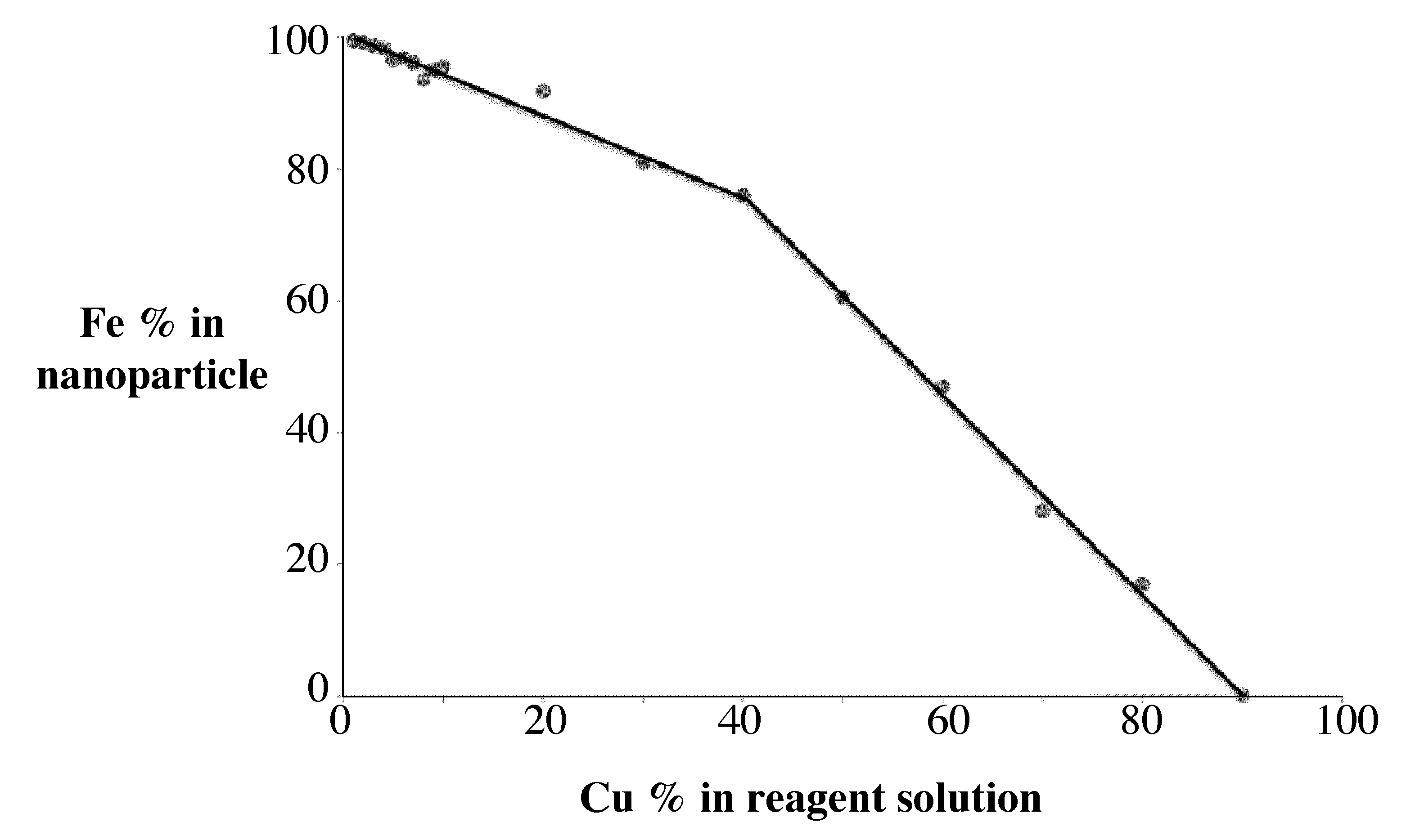
Subsequent \(\ce{Fe}\) and \(\ce{Cu}\) ICP-AES of the samples will allow the determination of \(\ce{Fe:Cu}\)ratio that is present in the nanoparticle. This can be compared to the ratio of \(\ce{Fe}\) and \(\ce{Cu}\)that was applied as reactants. The graph shows how the percentage of \(\ce{Fe}\) in the nanoparticle changes as a function of how much \(\ce{Fe}\) is used as a reagent.

Figure \(\PageIndex{2}\): Change in iron percentage in the Fe-Cu-O nanoparticles as a function of how much iron precursor is used in the synthesis of the nanoparticles.

Determining Analyte Concentration

Once the nanoparticles are digested and the ICP-AES analysis has been completed you must turn the figures from the ICP-AES analysis into working numbers to determine the concentration of metals in the solution that was synthesized initially.

Let's first consider the nanoparticles that are of one metal alone. The figure given by the analysis in this case is given in units of mg/L, this is the value in ppm's. This figure was recorded for the solution that was analyzed, and this is of a dilute concentration compared to the initial synthesized solution because the particles had to be digested in acid first, then diluted further into nanopure water.

As mentioned above in the experimental 0.5 mL of the synthesized nanoparticles were first digested in 9.5 mL of concentrated nitric acid. Then when the digestion was complete 0.5 mL of this solution was dissolved in 9.5 mL of nanopure water. This was the final solution that was analyzed using ICP, and the concentration of metal in this solution will be far lower than that of the original solution. In this case the amount of analyte in the final solution being analyzed is 1/20^th that of the total amount of material in the solution that was originally synthesized.

Calculating Concentration in ppm

Let us take an example that upon analysis by ICP-AES the amount of \(\ce{Fe}\) detected is 6.38 mg/L. First convert the figure to mg/mL,

\[ 6.38~\mathrm { mg } / \mathrm { L } \times 1 / 1000~\mathrm { L } / \mathrm { mL } = 6.38`\mathrm { x } 10 ^ { - 3 }~\mathrm { mg } / \mathrm { mL } \nonumber \]

The amount of material was diluted to a total volume of 10 mL. Therefore we should multiply this value by 10 mL to see how much mass was in the whole container.

\[ 6.38 \times 10 ^ { - 3 }~\mathrm { mg } / \mathrm { mL } \times 10~\mathrm { mL } = 6.38 \times 10 ^ { - 2 }~\mathrm { mg } \nonumber \]

This is the total mass of iron that was present in the solution that was analyzed using the ICP device. To convert this amount to ppm we should take into consideration the fact that 0.5 mL was initially diluted to 10 mL, to do this we should divide the total mass of iron by this amount that it was diluted to.

\[ 6.38 \times 10 ^ { - 2 }~\mathrm { mg } / 0.5~\mathrm { mL } = 0.1276~\mathrm { mg } / \mathrm { mL } \nonumber \]

This was the total amount of analyte in the 10 mL solution that was analyzed by the ICP device, to attain the value in ppm it should be mulitplied by a thousand, that is then 127.6 ppm of \(\ce{Fe}\).

Determining Concentration of Original Solution

We now need to factor in the fact that there were several dilutions of the original solution first to digest the metals and then to dissolve them in nanopure water, in all there were two dilutions and each dilution was equivalent in mass. By diluting 0.5 mL to 10 mL , we are effectively diluting the solution by a factor of 20, and this was carried out twice.

\[ 0.1276~\mathrm { mg } / \mathrm { mL } \times 20 = 2.552~\mathrm { mg } / \mathrm { mL } \nonumber \]

This is the amount of analyte in the solution of digested particles, to covert this to ppm we should multiply it by 1/1000 mL/L, in the following way:

\[ 2.552~\mathrm { mg } / \mathrm { mL } *\times 1 / 1000 \mathrm { mL } / \mathrm { L } = 2552~\mathrm { mg } / \mathrm { L } ^ { \mathrm { L } } \nonumber \]

This is essentially your answer now as 2552 ppm. This is the amount of \(\ce{Fe}\) in the solution of digested particles. This was made by diluting 0.5 mL of the original solution into 9.5 mL concentrated nitric acid, which is the same as diluting by a factor of 20. To calculate how much analyte was in the original batch that was synthesized we multiply the previous value by 20 again. This is the final amount of \(\ce{Fe}\) concentration of the original batch when it was synthesized and made soluble in hexanes.

\[ 2552~\mathrm { ppm } \times 20 = 51040~\mathrm { ppm } \nonumber \]

Calculating Stoichiometric Ratio

Moving from calculating the concentration of individual elements now we can concentrate on the calculation of stoichiometric ratios in the bi-metallic nanoparticles.

Consider the case when we have the iron and the copper elements in the nanoparticle. The amounts determined by ICP are:

• Iron = 1.429 mg/L.
• Copper = 1.837 mg/L.

We must account for the molecular weights of each element by dividing the ICP obtained value, by the molecular weight for that particular element. For iron this is calculated by

\[ \frac{1.429~\mathrm { mg }/ \mathrm { L }}{ 55.85} = 0.0211 \nonumber \],

and thus this is molar ratio of iron. On the other hand the ICP returns a value for copper that is given by:

\[ \frac{1.837 \mathrm { mg } / \mathrm { L } }{ 63.55} = 0.0289 \nonumber \]

To determine the percentage iron we use this equation, which gives a percentage value of 42.15% Fe.

\[ \% \text { Fe } = [ \frac{ \text { molar ratio of iron } }{\text { sum of molar ratios } } ] \times 100 \nonumber \]

We work out the copper percentage similarly, which leads to an answer of 57.85% Cu.

\[ \% \text { Cu} = [ \frac{ \text { molar ratio of copper} }{\text { sum of molar ratios } } ] \times 100 \nonumber \]

In this way the percentage iron in the nanoparticle can be determined as function of the reagent concentration prior to the synthesis (Figure \(\PageIndex{2}\) ).

Determining Concentration of Nanoparticles in Solution

The previous examples have shown how to calculate both the concentration of one analyte and the effective shared concentration of metals in the solution. These figures pertain to the concentration of elemental atoms present in solution. To use this to determine the concentration of nanoparticles we must first consider how many atoms that are being detected are in a nanoparticle. Let us consider that the \(\ce{Fe3O4}\) nanoparticles are of 7 nm diameter. In a 7 nm particle we expect to find 20,000 atoms. However in this analysis we have only detected Fe atoms, so we must still account for the number of oxygen atoms that form the crystal lattice also.

For every 3 Fe atoms, there are 4 O atoms. But as iron is slightly larger than oxygen, it will make up for the fact there is one less Fe atom. This is an over simplification but at this time it serves the purpose to make the reader aware of the steps that are required to take when judging nanoparticles concentration. Let us consider that half of the nanoparticle size is attributed to iron atoms, and the other half of the size is attributed to oxygen atoms.

As there are 20,000 atoms total in a 7 nm particle, and then when considering the effect of the oxide state we will say that for every 10,000 atoms of Fe you will have a 7 nm particle. So now we must find out how many Fe atoms are present in the sample so we can divide by 10,000 to determine how many nanoparticles are present.

In the case from above, we found the solution when synthesized had a concentration 51,040 ppm Fe atoms in solution. To determine how how many atoms this equates to we will use the fact that 1 mole of material has the Avogadro number of atoms present.

\[ 51040~\mathrm { ppm } = 51040~\mathrm { mg } / \mathrm { L } = 51.040~\mathrm { g } / \mathrm { L } \nonumber \]

1 mole of iron weighs 55.847 g. To determine how many moles we now have, we divide the values like this:

\[ \frac{ 51.040~\mathrm{g / L} }{ 55.847~\mathrm{g} } = 0.9139~\text { mol/L } \nonumber \]

The number of atoms is found by multiplying this by Avogadro’s number (6.022x10²³):

\[ ( 0.9139~\text { mol/L} ) \times \left( 6.022 \times 10 ^ { 23 } \text { atoms } \right) = 5.5 \times 10 ^ { 23 }~\text { atoms/L } \nonumber \]

For every 10,000 atoms we have a nanoparticle (NP) of 7 nm diameter, assuming all the particles are equivalent in size we can then divide the values. This is the concentration of nanoparticles per liter of solution as synthesized.

\[ \left( 5.5 \times 10 ^ { 23 } \text { atoms/ L } \right) / ( 10,000 \text { atoms/NP} ) = 5.5 \times 10 ^ { 19 }~\mathrm { NP } / \mathrm { L } \nonumber \]

Combined Surface Area

One very interesting thing about nanotechnology that nanoparticles can be used for is their incredible ratio between the surface areas compared with the volume. As the particles get smaller and smaller the surface area becomes more prominent. And as much of the chemistry is done on surfaces, nanoparticles are good contenders for future use where high aspect ratios are required.

In the example above we considered the particles to be of 7 nm diameters. The surface area of such a particle is 1.539 x10^-16 m². So the combined surface area of all the particles is found by multiplying each particle by their individual surface areas.

\[ \left( 1.539 \times 10 ^ { - 16 } \mathrm { m } ^ { 2 } \right) \times \left( 5.5 \times 10 ^ { 19 }~mathrm { NP } / \mathrm { L } \right) = 8465~\mathrm { m } ^ { 2 } / \mathrm { L } \nonumber \]

To put this into context, an American football field is approximately 5321 m². So a liter of this nanoparticle solution would have the same surface area of approximately 1.5 football fields. That is allot of area in one liter of solution when you consider how much material it would take to line the football field with thin layer of metallic iron. Remember there is only about 51 g/L of iron in this solution!

Bibliography

• http://www.ivstandards.com/extras/pertable/
• A. Scheffer, C. Engelhard, M. Sperling, and W. Buscher, W. Anal. Bioanal. Chem., 2008, 390, 249.
• H. Nakamuru, T. Shimizu, M. Uehara, Y. Yamaguchi, and H. Maeda, Mater. Res. Soc., Symp. Proc., 2007, 1056, 11.
• S. Sun and H. Zeng, J. Am. Chem. Soc., 2002, 124, 8204.
• C. A. Crouse and A. R. Barron, J. Mater. Chem., 2008, 18, 4146.