
8: Review of Chemical Kinetics
- Page ID
- 6653
\( \newcommand{\vecs}[1]{\overset { \scriptstyle \rightharpoonup} {\mathbf{#1}} } \)
\( \newcommand{\vecd}[1]{\overset{-\!-\!\rightharpoonup}{\vphantom{a}\smash {#1}}} \)
\( \newcommand{\dsum}{\displaystyle\sum\limits} \)
\( \newcommand{\dint}{\displaystyle\int\limits} \)
\( \newcommand{\dlim}{\displaystyle\lim\limits} \)
\( \newcommand{\id}{\mathrm{id}}\) \( \newcommand{\Span}{\mathrm{span}}\)
( \newcommand{\kernel}{\mathrm{null}\,}\) \( \newcommand{\range}{\mathrm{range}\,}\)
\( \newcommand{\RealPart}{\mathrm{Re}}\) \( \newcommand{\ImaginaryPart}{\mathrm{Im}}\)
\( \newcommand{\Argument}{\mathrm{Arg}}\) \( \newcommand{\norm}[1]{\| #1 \|}\)
\( \newcommand{\inner}[2]{\langle #1, #2 \rangle}\)
\( \newcommand{\Span}{\mathrm{span}}\)
\( \newcommand{\id}{\mathrm{id}}\)
\( \newcommand{\Span}{\mathrm{span}}\)
\( \newcommand{\kernel}{\mathrm{null}\,}\)
\( \newcommand{\range}{\mathrm{range}\,}\)
\( \newcommand{\RealPart}{\mathrm{Re}}\)
\( \newcommand{\ImaginaryPart}{\mathrm{Im}}\)
\( \newcommand{\Argument}{\mathrm{Arg}}\)
\( \newcommand{\norm}[1]{\| #1 \|}\)
\( \newcommand{\inner}[2]{\langle #1, #2 \rangle}\)
\( \newcommand{\Span}{\mathrm{span}}\) \( \newcommand{\AA}{\unicode[.8,0]{x212B}}\)
\( \newcommand{\vectorA}[1]{\vec{#1}} % arrow\)
\( \newcommand{\vectorAt}[1]{\vec{\text{#1}}} % arrow\)
\( \newcommand{\vectorB}[1]{\overset { \scriptstyle \rightharpoonup} {\mathbf{#1}} } \)
\( \newcommand{\vectorC}[1]{\textbf{#1}} \)
\( \newcommand{\vectorD}[1]{\overrightarrow{#1}} \)
\( \newcommand{\vectorDt}[1]{\overrightarrow{\text{#1}}} \)
\( \newcommand{\vectE}[1]{\overset{-\!-\!\rightharpoonup}{\vphantom{a}\smash{\mathbf {#1}}}} \)
\( \newcommand{\vecs}[1]{\overset { \scriptstyle \rightharpoonup} {\mathbf{#1}} } \)
\(\newcommand{\longvect}{\overrightarrow}\)
\( \newcommand{\vecd}[1]{\overset{-\!-\!\rightharpoonup}{\vphantom{a}\smash {#1}}} \)
\(\newcommand{\avec}{\mathbf a}\) \(\newcommand{\bvec}{\mathbf b}\) \(\newcommand{\cvec}{\mathbf c}\) \(\newcommand{\dvec}{\mathbf d}\) \(\newcommand{\dtil}{\widetilde{\mathbf d}}\) \(\newcommand{\evec}{\mathbf e}\) \(\newcommand{\fvec}{\mathbf f}\) \(\newcommand{\nvec}{\mathbf n}\) \(\newcommand{\pvec}{\mathbf p}\) \(\newcommand{\qvec}{\mathbf q}\) \(\newcommand{\svec}{\mathbf s}\) \(\newcommand{\tvec}{\mathbf t}\) \(\newcommand{\uvec}{\mathbf u}\) \(\newcommand{\vvec}{\mathbf v}\) \(\newcommand{\wvec}{\mathbf w}\) \(\newcommand{\xvec}{\mathbf x}\) \(\newcommand{\yvec}{\mathbf y}\) \(\newcommand{\zvec}{\mathbf z}\) \(\newcommand{\rvec}{\mathbf r}\) \(\newcommand{\mvec}{\mathbf m}\) \(\newcommand{\zerovec}{\mathbf 0}\) \(\newcommand{\onevec}{\mathbf 1}\) \(\newcommand{\real}{\mathbb R}\) \(\newcommand{\twovec}[2]{\left[\begin{array}{r}#1 \\ #2 \end{array}\right]}\) \(\newcommand{\ctwovec}[2]{\left[\begin{array}{c}#1 \\ #2 \end{array}\right]}\) \(\newcommand{\threevec}[3]{\left[\begin{array}{r}#1 \\ #2 \\ #3 \end{array}\right]}\) \(\newcommand{\cthreevec}[3]{\left[\begin{array}{c}#1 \\ #2 \\ #3 \end{array}\right]}\) \(\newcommand{\fourvec}[4]{\left[\begin{array}{r}#1 \\ #2 \\ #3 \\ #4 \end{array}\right]}\) \(\newcommand{\cfourvec}[4]{\left[\begin{array}{c}#1 \\ #2 \\ #3 \\ #4 \end{array}\right]}\) \(\newcommand{\fivevec}[5]{\left[\begin{array}{r}#1 \\ #2 \\ #3 \\ #4 \\ #5 \\ \end{array}\right]}\) \(\newcommand{\cfivevec}[5]{\left[\begin{array}{c}#1 \\ #2 \\ #3 \\ #4 \\ #5 \\ \end{array}\right]}\) \(\newcommand{\mattwo}[4]{\left[\begin{array}{rr}#1 \amp #2 \\ #3 \amp #4 \\ \end{array}\right]}\) \(\newcommand{\laspan}[1]{\text{Span}\{#1\}}\) \(\newcommand{\bcal}{\cal B}\) \(\newcommand{\ccal}{\cal C}\) \(\newcommand{\scal}{\cal S}\) \(\newcommand{\wcal}{\cal W}\) \(\newcommand{\ecal}{\cal E}\) \(\newcommand{\coords}[2]{\left\{#1\right\}_{#2}}\) \(\newcommand{\gray}[1]{\color{gray}{#1}}\) \(\newcommand{\lgray}[1]{\color{lightgray}{#1}}\) \(\newcommand{\rank}{\operatorname{rank}}\) \(\newcommand{\row}{\text{Row}}\) \(\newcommand{\col}{\text{Col}}\) \(\renewcommand{\row}{\text{Row}}\) \(\newcommand{\nul}{\text{Nul}}\) \(\newcommand{\var}{\text{Var}}\) \(\newcommand{\corr}{\text{corr}}\) \(\newcommand{\len}[1]{\left|#1\right|}\) \(\newcommand{\bbar}{\overline{\bvec}}\) \(\newcommand{\bhat}{\widehat{\bvec}}\) \(\newcommand{\bperp}{\bvec^\perp}\) \(\newcommand{\xhat}{\widehat{\xvec}}\) \(\newcommand{\vhat}{\widehat{\vvec}}\) \(\newcommand{\uhat}{\widehat{\uvec}}\) \(\newcommand{\what}{\widehat{\wvec}}\) \(\newcommand{\Sighat}{\widehat{\Sigma}}\) \(\newcommand{\lt}{<}\) \(\newcommand{\gt}{>}\) \(\newcommand{\amp}{&}\) \(\definecolor{fillinmathshade}{gray}{0.9}\)A reaction’s equilibrium position defines the extent to which the reaction can occur. For example, we expect a reaction with a large equilibrium constant, such as the dissociation of HCl in water
\[\ce{HCl}(aq) + \ce{H2O}(l) ⇋ \ce{H3O+}(aq) + \ce{Cl-}(aq) \nonumber \]
to proceed nearly to completion. A large equilibrium constant, however, does not guarantee that a reaction will reach its equilibrium position. Many reactions with large equilibrium constants, such as the reduction of MnO4– by H2O
\[\ce{4MnO4-}(aq) + \ce{2H2O}(l) ⇋ \ce{4MnO2}(s) + \ce{3O2}(g) + \ce{4OH-}(aq) \nonumber \]
do not occur to an appreciable extent. The study of the rate at which a chemical reaction approaches its equilibrium position is called kinetics.
A17.1 Chemical Reaction Rates
A study of a reaction’s kinetics begins with the measurement of its reaction rate. Consider, for example, the general reaction shown below, involving the aqueous solutes A, B, C, and D, with stoichiometries of a, b, c, and d.
\[a\ce{A} + b\ce{B} ⇋ c\ce{C} + d\ce{D}\tag{A17.1} \]
The rate, or velocity, at which this reaction approaches its equilibrium position is determined by following the change in concentration of one reactant or one product as a function of time. For example, if we monitor the concentration of reactant A, we express the rate as
\[R = -\dfrac{d[\ce A]}{dt}\tag{A17.2} \]
where R is the measured rate expressed as a change in concentration of A as a function of time. Because a reactant’s concentration decreases with time, we include a negative sign so that the rate has a positive value.
We also can determine the rate by following the change in concentration of a product as a function of time, which we express as
\[R´ = −\dfrac{d[\ce C]}{dt}\tag{A17.3} \]
Rates determined by monitoring different species do not necessarily have the same value. The rate R in equation A17.2 and the rate R´ in equation A17.3 have the same value only if the stoichiometric coefficients of A and C in reaction A17.1 are identical. In general, the relationship between the rates R and R´ is
\[R = \dfrac{a}{c} × R´ \nonumber \]
A17.2 The Rate Law
A rate law describes how a reaction’s rate is affected by the concentration of each species in the reaction mixture. The rate law for reaction A17.1 takes the general form of
\[R = k\mathrm{[A]^α[B]^β[C]^γ[D]^δ[E]^ε...}\tag{A17.4} \]
where k is the rate constant, and α, β, γ, δ, and ε are the reaction orders of the reaction for each species present in the reaction.
There are several important points about the rate law in equation A17.4. First, a reaction’s rate may depend on the concentrations of both reactants and products, as well as the concentration of a species that does not appear in the reaction’s overall stoichiometry. Species E in equation A17.4, for example, may be a catalyst that does not appear in the reaction’s overall stoichiometry, but which increases the reaction’s rate. Second, the reaction order for a given species is not necessarily the same as its stoichiometry in the chemical reaction. Reaction orders may be positive, negative, or zero, and may take integer or non-integer values. Finally, the reaction’s overall reaction order is the sum of the individual reaction orders for each species. Thus, the overall reaction order for equation A17.4 is α + β + γ + δ + ε.
A17.3 Kinetic Analysis of Selected Reactions
In this section we review the application of kinetics to several simple chemical reactions, focusing on how we can use the integrated form of the rate law to determine reaction orders. In addition, we consider how we can determine the rate law for a more complex system.
First-Order Reactions
The simplest case we can treat is a first-order reaction in which the reaction’s rate depends on the concentration of only one species. The best example of a first-order reaction is an irreversible thermal decomposition of a single reactant, which we represent as
\[\mathrm{A → Products}\tag{A17.5} \]
with a rate law of
\[R = -\dfrac{d[\ce A]}{dt} = k[\ce A]\tag{A17.6} \]
The simplest way to demonstrate that a reaction is first-order in A, is to double the concentration of A and note the effect on the reaction’s rate. If the observed rate doubles, then the reaction must be first-order in A. Alternatively, we can derive a relationship between the concentration of A and time by rearranging equation A17.6 and integrating.
\[\dfrac{d[\ce A]}{[\ce A]} = -k dt \nonumber \]
\[\int_{[\ce A]_0}^{[\ce A]_t} \dfrac{d[\ce A]}{[\ce A]} = -k \int_{0}^{t}dt\tag{A17.7} \]
Evaluating the integrals in equation A17.7 and rearranging
\[\ln\dfrac{[\ce A]_t}{[\ce A]_0}= -kt\tag{A17.8} \]
\[\ln[\ce A]_t = -kt+ \ln[\ce A]_0\tag{A17.9} \]
shows that for a first-order reaction, a plot of ln[A]t versus time is linear with a slope of –k and a y-intercept of ln[A]0. Equation A17.8 and equation A17.9 are known as integrated forms of the rate law.
Reaction A17.5 is not the only possible form of a first-order reaction. For example, the reaction
\[\mathrm{A + B → Products}\tag{A17.10} \]
will follow first-order kinetics if the reaction is first-order in A and if the concentration of B does not affect the reaction’s rate. This may happen if the reaction’s mechanism involves at least two steps. Imagine that in the first step, A slowly converts to an intermediate species, C, which rapidly reacts with the remaining reactant, B, in one or more steps, to form the products.
\[\mathrm{A → B \hspace{20px}(slow)} \nonumber \]
\[\mathrm{B + C → Products \hspace{20px} (fast)} \nonumber \]
Because a reaction’s rate depends only on those species in the slowest step—usually called the rate-determining step—and any preceding steps, species B will not appear in the rate law.
Second-Order Reactions
The simplest reaction demonstrating second-order behavior is
\[\mathrm{2A → Products} \nonumber \]
for which the rate law is
\[R = -\dfrac{d[\ce A]}{dt}= k[\ce A]^2 \nonumber \]
Proceeding as we did earlier for a first-order reaction, we can easily derive the integrated form of the rate law.
\[\dfrac{d[\ce A]}{[\ce A]^2}= -k\, dt \nonumber \]
\[\int_{[\ce A]_0}^{[\ce A]_t} \dfrac{d[\ce A]}{[\ce A]^2} = -k \int_{0}^{t}dt \nonumber \]
\[\dfrac{1}{[\ce A]_t} = kt + \dfrac{1}{[\ce A]_0} \nonumber \]
For a second-order reaction, therefore, a plot of [A]t–1 versus t is linear with a slope of k and a y-intercept of [A]0–1. Alternatively, we can show that a reaction is second-order in A by observing the effect on the rate when we change the concentration of A. In this case, doubling the concentration of A produces a four-fold increase in the reaction’s rate.
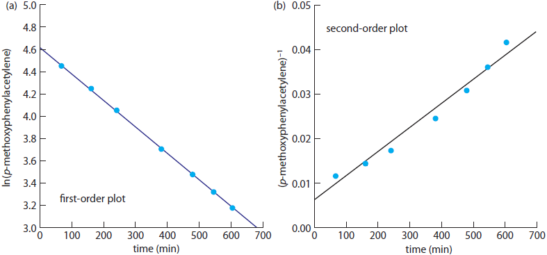
The following data were obtained during a kinetic study of the hydration of p-methoxyphenylacetylene by measuring the relative amounts of reactants and products by NMR.1
|
time (min) |
% p-methyoxyphenylacetylene |
|
67 |
85.9 |
|
161 |
70.0 |
|
241 |
57.6 |
|
381 |
40.7 |
|
479 |
32.4 |
|
545 |
27.7 |
|
604 |
24 |
Determine whether this reaction is first-order or second-order in p-methoxyphenylacetylene.
Solution
To determine the reaction’s order we plot ln(%pmethoxyphenylacetylene) versus time for a first-order reaction, and (%p-methoxyphenylacetylene)–1 versus time for a second-order reaction (see Figure A17.1). Because a straight-line for the first-order plot fits the data nicely, we conclude that the reaction is first-order in p-methoxyphenylacetylene. Note that when we plot the data using the equation for a second-order reaction, the data show curvature that does not fit the straight-line model.
Pseudo-Order Reactions and the Method of Initial Rates
Unfortunately, most reactions of importance in analytical chemistry do not follow the simple first-order or second-order rate laws discussed above. We are more likely to encounter the second-order rate law given in equation A17.11 than that in equation A17.10.
\[R = k\mathrm{[A][B]}\tag{A17.11} \]
Demonstrating that a reaction obeys the rate law in equation A17.11 is complicated by the lack of a simple integrated form of the rate law. Often we can simplify the kinetics by carrying out the analysis under conditions where the concentrations of all species but one are so large that their concentrations remain effectively constant during the reaction. For example, if the concentration of B is selected such that [B] >> [A], then equation A17.11 simplifies to
\[R = k´[\ce A] \nonumber \]
where the rate constant k´ is equal to k[B]. Under these conditions, the reaction appears to follow first-order kinetics in A and, for this reason we identify the reaction as pseudo-first-order in A. We can verify the reaction order for A using either the integrated rate law or by observing the effect on the reaction’s rate of changing the concentration of A. To find the reaction order for B, we repeat the process under conditions where [A] >> [B].
A variation on the use of pseudo-ordered reactions is the initial rate method. In this approach we run a series of experiments in which we change one at a time the concentration of those species expected to affect the reaction’s rate and measure the resulting initial rate. Comparing the reaction’s initial rate for two experiments in which only the concentration of one species is different allows us to determine the reaction order for that species. The application of this method is outlined in the following example.
The following data was collected during a kinetic study of the iodation of acetone by measuring the concentration of unreacted I2 in solution.2
|
experiment number |
[C3H6O] (M) |
[H3O+] (M) |
[I2] (M) |
Rate (M s–1) |
|
1 |
1.33 |
0.0404 |
6.65×10⁻³ |
1.78×10⁻⁶ |
|
2 |
1.33 |
0.0809 |
6.65×10⁻³ |
3.89×10⁻⁶ |
|
3 |
1.33 |
0.162 |
6.65×10⁻³ |
8.11×10⁻⁶ |
|
4 |
1.33 |
0.323 |
6.65×10⁻³ |
1.66×10⁻⁵ |
|
5 |
0.167 |
0.323 |
6.65×10⁻³ |
1.64×10⁻⁶ |
|
6 |
0.333 |
0.323 |
6.65×10⁻³ |
3.76×10⁻⁶ |
|
7 |
0.667 |
0.323 |
6.65×10⁻³ |
7.55×10⁻⁶ |
|
8 |
0.333 |
0.323 |
3.32×10⁻³ |
3.57×10⁻⁶ |
Solution
The order of the rate law with respect to the three reactants is determined by comparing the rates of two experiments in which there is a change in concentration for only one of the reactants. For example, in experiment 2 the [H3O+] and the rate are approximately twice as large as in experiment 1, indicating that the reaction is first-order in [H3O+]. Working in the same manner, experiments 6 and 7 show that the reaction is also first order with respect to [C3H6O], and experiments 6 and 8 show that the rate of the reaction is independent of the [I2]. Thus, the rate law is
\[R = k\ce{[C3H6O][H3O+]} \nonumber \]
To determine the value of the rate constant, we substitute the rate, the [C3H6O], and the [H3O+] for each experiment into the rate law and solve for k. Using the data from experiment 1, for example, gives a rate constant of 3.31×10⁻⁵ M–1 sec–1. The average rate constant for the eight experiments is 3.49×10⁻⁵ M–1 sec–1.
References
- Kaufman, D,; Sterner, C.; Masek, B.; Svenningsen, R.; Samuelson, G. J. Chem. Educ. 1982, 59, 885–886.
- Birk, J. P.; Walters, D. L. J. Chem. Educ. 1992, 69, 585–587.