10.4: The Clausius-Clapeyron Equation

Evaporation

In Section 23.3, the Clapeyron Equation was derived for melting points.

$$\dfrac{dP}{dT} = \dfrac{ΔH_{molar}}{TΔV_{molar}} \nonumber$$

However, our argument is actually quite general and should hold for vapor equilibria as well. The only problem is that the molar volume of gases are by no means so nicely constant as they are for condensed phases. (i. e., for condenses phases, both $α$ and $κ$ are pretty small).

We can write:

$$\dfrac{dP}{dT} =\dfrac{ ΔH_{molar}}{TΔV_{molar}} = \dfrac{ΔH_{molar}}{T} \left[V_{molar}^{gas}-V_{molar}^{liquid} \right] \nonumber$$

as

$$V_{molar}^{gas} \gg V_{molar}^{liquid} \nonumber$$

we can approximate

$$V_{molar}^{gas}-V_{molar}^{liquid} \nonumber$$

by just taking $V_{molar}^{gas}$. Further more if the vapor is considered an ideal gas, then

$$V_{molar}^{gas} = \dfrac{RT}{P} \nonumber$$

We get

$$\dfrac{1}{P} .\dfrac{dP}{dT} = \dfrac{d \ln P}{dT} = \dfrac{ΔH_{molar}^{vap}}{RT^2} \label{CCe}$$

Equation $\ref{CCe}$ is known as the Clausius-Clapeyron equation. We can further work our the integration and find the how the equilibrium vapor pressure changes with temperature:

$$\ln \left( \dfrac{P_2}{P_1} \right)= \dfrac{-ΔH_{molar}^{vap}}{R} \left[\dfrac{1}{T_2}-\dfrac{1}{T_1} \right] \nonumber$$

Thus if we know the molar enthalpy of vaporization we can predict the vapor lines in the diagram. Of course the approximations made are likely to lead to deviations if the vapor is not ideal or very dense (e.g., approaching the critical point).

The Clapeyron Equation

The Clapeyron attempts to answer the question of what the shape of a two-phase coexistence line is. In the $P-T$ plane, we see the a function $P(T)$, which gives us the dependence of $P$ on $T$ along a coexistence curve.

Consider two phases, denoted $\alpha$ and $\beta$, in equilibrium with each other. These could be solid and liquid, liquid and gas, solid and gas, two solid phases, et. Let $\mu_\alpha (P, T)$ and $\mu_\beta (P, T)$ be the chemical potentials of the two phases. We have just seen that

$$\mu_\alpha (P, T) = \mu_\beta (P, T) \label{14.1}$$

Next, suppose that the pressure and temperature are changed by $dP$ and $dT$. The changes in the chemical potentials of each phase are

$$d \mu_{\alpha} (P, T) = d \mu_{\beta} (P, T) \label{14.2a}$$

$$\left( \dfrac{\partial \mu_{\alpha}}{\partial P} \right)_T dP + \left( \dfrac{\partial \mu_{\alpha}}{\partial T} \right)_P dT = \left( \dfrac{\partial \mu_{\beta}}{\partial P} \right)_T dP + \left( \dfrac{\partial \mu_{\beta}}{\partial T} \right)_P dT \label{14.2b}$$

However, since $G(n, P, T) = n \mu (P, T)$, the molar free energy $\bar{G} (P, T)$, which is $G(n, P, T)/n$, is also just equal to the chemical potential

$$\bar{G} (P, T) = \dfrac{G(n, P, T)}{n} = \mu (P, T) \label{14.3}$$

Moreover, the derivatives of $\bar{G}$ are

$$\left( \dfrac{\partial \bar{G}}{\partial P} \right)_T = \bar{V}, \: \: \: \: \: \: \: \left( \dfrac{\partial \bar{G}}{\partial T} \right)_P = -\bar{S} \label{14.4}$$

Applying these results to the chemical potential condition in Equation $\ref{14.2b}$, we obtain

$$\begin{align} \left( \dfrac{\partial \bar{G}_\alpha}{\partial P} \right)_T dP + \left( \dfrac{\partial \bar{G}_\alpha}{\partial T} \right)_P dT &= \left( \dfrac{\partial \bar{G}_\beta}{\partial P} \right)_T dP + \left( \dfrac{\partial \bar{G}_\beta}{\partial T} \right)_P dT \\[5pt] \bar{V}_\alpha dP - \bar{S}_\alpha dT &= \bar{V}_\beta dP - \bar{S}_\beta dT \end{align} \label{14.5}$$

Dividing through by $dT$, we obtain

$$\begin{align} \bar{V}_\alpha \dfrac{\partial P}{\partial T} - \bar{S}_\alpha &= \bar{V}_\beta \dfrac{\partial P}{\partial T} - \bar{S}_\beta \\[5pt] (\bar{V}_\alpha - \bar{V}_\beta) \dfrac{\partial P}{\partial T} &= \bar{S}_\alpha - \bar{S}_\beta \\[5pt] \dfrac{dP}{dT} &= \dfrac{\bar{S}_\alpha - \bar{S}_\beta}{\bar{V}_\alpha - \bar{V}_\beta} \end{align} \label{14.6}$$

The importance of the quantity $dP/dT$ is that is represents the slope of the coexistence curve on the phase diagram between the two phases. Now, in equilibrium $dG = 0$, and since $G = H - TS$, it follows that $dH = T \: dS$ at fixed $T$. In the narrow temperature range in which the two phases are in equilibrium, we can assume that $H$ is independent of $T$, hence, we can write $S = H/T$. Consequently, we can write the molar entropy difference as

$$\bar{S}_\alpha - \bar{S}_\beta = \dfrac{\bar{H}_\alpha - \bar{H}_\beta}{T} \label{14.7}$$

and the pressure derivative $dP/dT$ becomes

$$\dfrac{dP}{dT} = \dfrac{\bar{H}_\alpha - \bar{H}_\beta}{T (\bar{V}_\alpha - \bar{V}_\beta)} = \dfrac{\Delta_{\alpha \beta} \bar{H}}{T \Delta_{\alpha \beta} \bar{V}} \label{14.8}$$

a result known as the Clapeyron equation, which tells us that the slope of the coexistence curve is related to the ratio of the molar enthalpy between the phases to the change in the molar volume between the phases. If the phase equilibrium is between the solid and liquid phases, then $\Delta_{\alpha \beta} \bar{H}$ and $\Delta_{\alpha \beta} \bar{V}$ are $\Delta \bar{H}_\text{fus}$ and $\Delta \bar{V}_\text{fus}$, respectively. If the phase equilibrium is between the liquid and gas phases, then $\Delta_{\alpha \beta} \bar{H}$ and $\Delta_{\alpha \beta} \bar{V}$ are $\Delta \bar{H}_\text{vap}$ and $\Delta \bar{V}_\text{vap}$, respectively.

For the liquid-gas equilibrium, some interesting approximations can be made in the use of the Clapeyron equation. For this equilibrium, Equation $\ref{14.8}$ becomes

$$\dfrac{dP}{dT} = \dfrac{\Delta \bar{H}_\text{vap}}{T (\bar{V}_g - \bar{V}_l)} \label{14.9}$$

In this case, $\bar{V}_g \gg \bar{V}_l$, and we can approximate Equation $\ref{14.9}$ as

$$\dfrac{dP}{dT} \approx \dfrac{\Delta \bar{H}_\text{vap}}{T \bar{V}_g} \label{14.10}$$

Suppose that we can treat the vapor phase as an ideal gas. Certainly, this is not a good approximation so close to the vaporization point, but it leads to an example we can integrate. Since $PV_g = nRT$, $P \bar{V}_g = RT$, Equation $\ref{14.10}$ becomes

$$\begin{align} \dfrac{dP}{dT} &= \dfrac{\Delta \bar{H}_\text{vap} P}{RT^2} \\[5pt] \dfrac{1}{P} \dfrac{dP}{dT} &= \dfrac{\Delta \bar{H}_\text{vap}}{RT^2} \\[5pt] \dfrac{d \: \text{ln} \: P}{dT} &= \dfrac{\Delta \bar{H}_\text{vap}}{RT^2} \end{align} \label{14.11}$$

which is called the Clausius-Clapeyron equation. We now integrate both sides, which yields

$$\text{ln} \: P = -\dfrac{\Delta \bar{H}_\text{vap}}{RT} + C \nonumber$$

where $C$ is a constant of integration. Exponentiating both sides, we find

$$P(T) = C' e^{-\Delta \bar{H}_\text{vap}/RT} \nonumber$$

which actually has the wrong curvature for large $T$, but since the liquid-vapor coexistence line terminates in a critical point, as long as $T$ is not too large, the approximation leading to the above expression is not that bad.

If we, instead, integrate both sides, the left from $P_1$ to $P_2$, and the right from $T_1$ to $T_2$, we find

$$\begin{align} \int_{P_1}^{P_2} d \: \text{ln} \: P &= \int_{T_1}^{T_2} \dfrac{\Delta \bar{H}_\text{vap}}{RT^2} dT \\[5pt] \text{ln} \: \left( \dfrac{P_2}{P_1} \right) &= -\dfrac{\Delta \bar{H}_\text{vap}}{R} \left( \dfrac{1}{T_2} - \dfrac{1}{T_1} \right) \\[5pt] &= \dfrac{\Delta \bar{H}_\text{vap}}{R} \left( \dfrac{T_1 - T_1}{T_1 T_2} \right) \end{align} \label{14.12}$$

assuming that $\Delta \bar{H}_\text{vap}$ is independent of $T$. Here $P_1$ is the pressure of the liquid phase, and $P_2$ is the pressure of the vapor phase. Suppose we know $P_2$ at a temperature $T_2$, and we want to know $P_3$ at another temperature $T_3$. The above result can be written as

$$\text{ln} \: \left( \dfrac{P_3}{P_1} \right) = -\dfrac{\Delta \bar{H}_\text{vap}}{R} \left( \dfrac{1}{T_3} - \dfrac{1}{T_1} \right) \label{14.13}$$

Subtracting the two results, we obtain

$$\text{ln} \: \left( \dfrac{P_2}{P_3} \right) = -\dfrac{\Delta \bar{H}_\text{vap}}{R} \left( \dfrac{1}{T_2} - \dfrac{1}{T_3} \right) \label{14.14}$$

so that we can determine the vapor pressure at any temperature if it is known as one temperature.

In order to illustrate the use of this result, consider the following example:

Example 23.4.1

At $1 \: \text{bar}$, the boiling point of water is $373 \: \text{K}$. At what pressure does water boil at $473 \: \text{K}$? Take the heat of vaporization of water to be $40.65 \: \text{kJ/mol}$.

Solution

Let $P_1 = 1 \: \text{bar}$ and $T_1 = 373 \: \text{K}$. Take $T_2 = 473 \: \text{K}$, and we need to calculate $P_2$. Substituting in the numbers, we find

$$\begin{align} \text{ln} \: P_2(\text{bar}) &= -\dfrac{(40.65 \: \text{kJ/mol})(1000 \: \text{J/kJ})}{8.3145 \: \text{J/mol} \cdot \text{K}} \left( \dfrac{1}{473 \: \text{K}} - \dfrac{1}{373 \: \text{K}} \right) = 2.77 \\[5pt] P_2(\text{bar}) &= (1 \: \text{bar}) \: e^{2.77} = 16 \: \text{bar} \end{align} \nonumber$$

Learning Objectives

• Apply the Clausius-Clapeyron equation to estimate the vapor pressure at any temperature.
• Estimate the heat of phase transition from the vapor pressures measured at two temperatures.

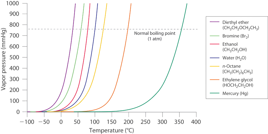
The vaporization curves of most liquids have similar shapes with the vapor pressure steadily increasing as the temperature increases (Figure $\PageIndex{1}$).

Figure $\PageIndex{1}$: The Vapor Pressures of Several Liquids as a Function of Temperature. The point at which the vapor pressure curve crosses the P = 1 atm line (dashed) is the normal boiling point of the liquid. (CC BY-SA-NC 3.0; Anonymous)

A good approach is to find a mathematical model for the pressure increase as a function of temperature. Experiments showed that the vapor pressure $P$ and temperature $T$ are related,

$$P \propto \exp \left(- \dfrac{\Delta H_{vap}}{RT}\right) \ \label{1}$$

where $\Delta{H_{vap}}$ is the Enthalpy (heat) of Vaporization and $R$ is the gas constant (8.3145 J mol^-1 K^-1).

A simple relationship can be found by integrating Equation $\ref{1}$ between two pressure-temperature endpoints:

$$\ln \left( \dfrac{P_1}{P_2} \right) = \dfrac{\Delta H_{vap}}{R} \left( \dfrac{1}{T_2}- \dfrac{1}{T_1} \right) \label{2}$$

where $P_1$ and $P_2$ are the vapor pressures at two temperatures $T_1$ and $T_2$. Equation $\ref{2}$ is known as the Clausius-Clapeyron Equation and allows us to estimate the vapor pressure at another temperature, if the vapor pressure is known at some temperature, and if the enthalpy of vaporization is known.

Alternative Formulation

The order of the temperatures in Equation $\ref{2}$ matters as the Clausius-Clapeyron Equation is sometimes written with a negative sign (and switched order of temperatures):

$$\ln \left( \dfrac{P_1}{P_2} \right) = - \dfrac{\Delta H_{vap}}{R} \left( \dfrac{1}{T_1}- \dfrac{1}{T_2} \right) \label{2B}$$

Example $\PageIndex{1}$: Vapor Pressure of Water

The vapor pressure of water is 1.0 atm at 373 K, and the enthalpy of vaporization is 40.7 kJ mol^-1. Estimate the vapor pressure at temperature 363 and 383 K respectively.

Solution

Using the Clausius-Clapeyron equation (Equation $\ref{2B}$), we have:

$$\begin{align} P_{363} &= 1.0 \exp \left[- \left(\dfrac{40,700}{8.3145}\right) \left(\dfrac{1}{363\;K} -\dfrac{1}{373\; K}\right) \right] \nonumber \\[4pt] &= 0.697\; atm \nonumber \end{align} \nonumber$$

$$\begin{align} P_{383} &= 1.0 \exp \left[- \left( \dfrac{40,700}{8.3145} \right)\left(\dfrac{1}{383\;K} - \dfrac{1}{373\;K} \right) \right] \nonumber \\[4pt] &= 1.409\; atm \nonumber \end{align} \nonumber$$

Note that the increase in vapor pressure from 363 K to 373 K is 0.303 atm, but the increase from 373 to 383 K is 0.409 atm. The increase in vapor pressure is not a linear process.

Discussion

We can use the Clausius-Clapeyron equation to construct the entire vaporization curve. There is a deviation from experimental value, that is because the enthalpy of vaporization varies slightly with temperature.

The Clausius-Clapeyron equation can be also applied to sublimation; the following example shows its application in estimating the heat of sublimation.

Example $\PageIndex{2}$: Sublimation of Ice

The vapor pressures of ice at 268 K and 273 K are 2.965 and 4.560 torr respectively. Estimate the heat of sublimation of ice.

Solution

The enthalpy of sublimation is $\Delta{H}_{sub}$. Use a piece of paper and derive the Clausius-Clapeyron equation so that you can get the form:

$$\begin{align} \Delta H_{sub} &= \dfrac{ R \ln \left(\dfrac{P_{273}}{P_{268}}\right)}{\dfrac{1}{268 \;K} - \dfrac{1}{273\;K}} \nonumber \\[4pt] &= \dfrac{8.3145 \ln \left(\dfrac{4.560}{2.965} \right)}{ \dfrac{1}{268\;K} - \dfrac{1}{273\;K} } \nonumber \\[4pt] &= 52,370\; J\; mol^{-1}\nonumber \end{align} \nonumber$$

Note that the heat of sublimation is the sum of heat of melting (6,006 J/mol at 0°C and 101 kPa) and the heat of vaporization (45,051 J/mol at 0 °C).

Exercise $\PageIndex{2}$

Show that the vapor pressure of ice at 274 K is higher than that of water at the same temperature. Note the curve of vaporization is also called the curve of evaporization.

Example $\PageIndex{3}$: Vaporization of Ethanol

Calculate $\Delta{H_{vap}}$ for ethanol, given vapor pressure at 40 ^oC = 150 torr. The normal boiling point for ethanol is 78 ^oC.

Solution

Recognize that we have TWO sets of $(P,T)$ data:

• Set 1: (150 torr at 40+273K)
• Set 2: (760 torr at 78+273K)

We then directly use these data in Equation $\ref{2B}$

$$\begin{align*} \ln \left(\dfrac{150}{760} \right) &= \dfrac{-\Delta{H_{vap}}}{8.314} \left[ \dfrac{1}{313} - \dfrac{1}{351}\right] \\[4pt] \ln 150 -\ln 760 &= \dfrac{-\Delta{H_{vap}}}{8.314} \left[ \dfrac{1}{313} - \dfrac{1}{351}\right] \\[4pt] -1.623 &= \dfrac{-\Delta{H_{vap}}}{8.314} \left[ 0.0032 - 0.0028 \right] \end{align*}$$

Then solving for $\Delta{H_{vap}}$

$$\begin{align*} \Delta{H_{vap}} &= 3.90 \times 10^4 \text{ joule/mole} \\[4pt] &= 39.0 \text{ kJ/mole} \end{align*}$$

Advanced Note

It is important to not use the Clausius-Clapeyron equation for the solid to liquid transition. That requires the use of the more general Clapeyron equation

$$\dfrac{dP}{dT} = \dfrac{\Delta \bar{H}}{T \Delta \bar{V}} \nonumber$$

where $\Delta \bar{H}$ and $\Delta \bar{V}$ is the molar change in enthalpy (the enthalpy of fusion in this case) and volume respectively between the two phases in the transition.