
12.7: Electrophoresis
- Page ID
- 5599

\( \newcommand{\vecs}[1]{\overset { \scriptstyle \rightharpoonup} {\mathbf{#1}} } \)
\( \newcommand{\vecd}[1]{\overset{-\!-\!\rightharpoonup}{\vphantom{a}\smash {#1}}} \)
\( \newcommand{\id}{\mathrm{id}}\) \( \newcommand{\Span}{\mathrm{span}}\)
( \newcommand{\kernel}{\mathrm{null}\,}\) \( \newcommand{\range}{\mathrm{range}\,}\)
\( \newcommand{\RealPart}{\mathrm{Re}}\) \( \newcommand{\ImaginaryPart}{\mathrm{Im}}\)
\( \newcommand{\Argument}{\mathrm{Arg}}\) \( \newcommand{\norm}[1]{\| #1 \|}\)
\( \newcommand{\inner}[2]{\langle #1, #2 \rangle}\)
\( \newcommand{\Span}{\mathrm{span}}\)
\( \newcommand{\id}{\mathrm{id}}\)
\( \newcommand{\Span}{\mathrm{span}}\)
\( \newcommand{\kernel}{\mathrm{null}\,}\)
\( \newcommand{\range}{\mathrm{range}\,}\)
\( \newcommand{\RealPart}{\mathrm{Re}}\)
\( \newcommand{\ImaginaryPart}{\mathrm{Im}}\)
\( \newcommand{\Argument}{\mathrm{Arg}}\)
\( \newcommand{\norm}[1]{\| #1 \|}\)
\( \newcommand{\inner}[2]{\langle #1, #2 \rangle}\)
\( \newcommand{\Span}{\mathrm{span}}\) \( \newcommand{\AA}{\unicode[.8,0]{x212B}}\)
\( \newcommand{\vectorA}[1]{\vec{#1}} % arrow\)
\( \newcommand{\vectorAt}[1]{\vec{\text{#1}}} % arrow\)
\( \newcommand{\vectorB}[1]{\overset { \scriptstyle \rightharpoonup} {\mathbf{#1}} } \)
\( \newcommand{\vectorC}[1]{\textbf{#1}} \)
\( \newcommand{\vectorD}[1]{\overrightarrow{#1}} \)
\( \newcommand{\vectorDt}[1]{\overrightarrow{\text{#1}}} \)
\( \newcommand{\vectE}[1]{\overset{-\!-\!\rightharpoonup}{\vphantom{a}\smash{\mathbf {#1}}}} \)
\( \newcommand{\vecs}[1]{\overset { \scriptstyle \rightharpoonup} {\mathbf{#1}} } \)
\( \newcommand{\vecd}[1]{\overset{-\!-\!\rightharpoonup}{\vphantom{a}\smash {#1}}} \)
\(\newcommand{\avec}{\mathbf a}\) \(\newcommand{\bvec}{\mathbf b}\) \(\newcommand{\cvec}{\mathbf c}\) \(\newcommand{\dvec}{\mathbf d}\) \(\newcommand{\dtil}{\widetilde{\mathbf d}}\) \(\newcommand{\evec}{\mathbf e}\) \(\newcommand{\fvec}{\mathbf f}\) \(\newcommand{\nvec}{\mathbf n}\) \(\newcommand{\pvec}{\mathbf p}\) \(\newcommand{\qvec}{\mathbf q}\) \(\newcommand{\svec}{\mathbf s}\) \(\newcommand{\tvec}{\mathbf t}\) \(\newcommand{\uvec}{\mathbf u}\) \(\newcommand{\vvec}{\mathbf v}\) \(\newcommand{\wvec}{\mathbf w}\) \(\newcommand{\xvec}{\mathbf x}\) \(\newcommand{\yvec}{\mathbf y}\) \(\newcommand{\zvec}{\mathbf z}\) \(\newcommand{\rvec}{\mathbf r}\) \(\newcommand{\mvec}{\mathbf m}\) \(\newcommand{\zerovec}{\mathbf 0}\) \(\newcommand{\onevec}{\mathbf 1}\) \(\newcommand{\real}{\mathbb R}\) \(\newcommand{\twovec}[2]{\left[\begin{array}{r}#1 \\ #2 \end{array}\right]}\) \(\newcommand{\ctwovec}[2]{\left[\begin{array}{c}#1 \\ #2 \end{array}\right]}\) \(\newcommand{\threevec}[3]{\left[\begin{array}{r}#1 \\ #2 \\ #3 \end{array}\right]}\) \(\newcommand{\cthreevec}[3]{\left[\begin{array}{c}#1 \\ #2 \\ #3 \end{array}\right]}\) \(\newcommand{\fourvec}[4]{\left[\begin{array}{r}#1 \\ #2 \\ #3 \\ #4 \end{array}\right]}\) \(\newcommand{\cfourvec}[4]{\left[\begin{array}{c}#1 \\ #2 \\ #3 \\ #4 \end{array}\right]}\) \(\newcommand{\fivevec}[5]{\left[\begin{array}{r}#1 \\ #2 \\ #3 \\ #4 \\ #5 \\ \end{array}\right]}\) \(\newcommand{\cfivevec}[5]{\left[\begin{array}{c}#1 \\ #2 \\ #3 \\ #4 \\ #5 \\ \end{array}\right]}\) \(\newcommand{\mattwo}[4]{\left[\begin{array}{rr}#1 \amp #2 \\ #3 \amp #4 \\ \end{array}\right]}\) \(\newcommand{\laspan}[1]{\text{Span}\{#1\}}\) \(\newcommand{\bcal}{\cal B}\) \(\newcommand{\ccal}{\cal C}\) \(\newcommand{\scal}{\cal S}\) \(\newcommand{\wcal}{\cal W}\) \(\newcommand{\ecal}{\cal E}\) \(\newcommand{\coords}[2]{\left\{#1\right\}_{#2}}\) \(\newcommand{\gray}[1]{\color{gray}{#1}}\) \(\newcommand{\lgray}[1]{\color{lightgray}{#1}}\) \(\newcommand{\rank}{\operatorname{rank}}\) \(\newcommand{\row}{\text{Row}}\) \(\newcommand{\col}{\text{Col}}\) \(\renewcommand{\row}{\text{Row}}\) \(\newcommand{\nul}{\text{Nul}}\) \(\newcommand{\var}{\text{Var}}\) \(\newcommand{\corr}{\text{corr}}\) \(\newcommand{\len}[1]{\left|#1\right|}\) \(\newcommand{\bbar}{\overline{\bvec}}\) \(\newcommand{\bhat}{\widehat{\bvec}}\) \(\newcommand{\bperp}{\bvec^\perp}\) \(\newcommand{\xhat}{\widehat{\xvec}}\) \(\newcommand{\vhat}{\widehat{\vvec}}\) \(\newcommand{\uhat}{\widehat{\uvec}}\) \(\newcommand{\what}{\widehat{\wvec}}\) \(\newcommand{\Sighat}{\widehat{\Sigma}}\) \(\newcommand{\lt}{<}\) \(\newcommand{\gt}{>}\) \(\newcommand{\amp}{&}\) \(\definecolor{fillinmathshade}{gray}{0.9}\)Electrophoresis is a class of separation techniques in which we separate analytes by their ability to move through a conductive medium—usually an aqueous buffer—in response to an applied electric field. In the absence of other effects, cations migrate toward the electric field’s negatively charged cathode. Cations with larger charge-to-size ratios—which favors ions of larger charge and of smaller size—migrate at a faster rate than larger cations with smaller charges. Anions migrate toward the positively charged anode and neutral species do not experience the electrical field and remain stationary.
There are several forms of electrophoresis. In slab gel electrophoresis the conducting buffer is retained within a porous gel of agarose or polyacrylamide. Slabs are formed by pouring the gel between two glass plates separated by spacers. Typical thicknesses are 0.25–1 mm. Gel electrophoresis is an important technique in biochemistry where it is frequently used for separating DNA fragments and proteins. Although it is a powerful tool for the qualitative analysis of complex mixtures, it is less useful for quantitative work.
In capillary electrophoresis, the conducting buffer is retained within a capillary tube whose inner diameter is typically 25–75 μm. Samples are injected into one end of the capillary tube. As the sample migrates through the capillary its components separate and elute from the column at different times. The resulting electropherogram looks similar to a GC or an HPLC chromatogram, providing both qualitative and quantitative information. Only capillary electrophoretic methods receive further consideration in this section.
As we will see shortly, under normal conditions even neutral species and anions migrate toward the cathode.
12.7.1 Theory of Capillary Electrophoresis
In capillary electrophoresis we inject the sample into a buffered solution retained within a capillary tube. When an electric field is applied across the capillary tube, the sample’s components migrate as the result of two types of action: electrophoretic mobility and electroosmotic mobility. Electrophoretic mobility is the solute’s response to the applied electrical field. As described earlier, cations move toward the negatively charged cathode, anions move toward the positively charged anode, and neutral species remain stationary. The other contribution to a solute’s migration is electroosmotic flow, which occurs when the buffer moves through the capillary in response to the applied electrical field. Under normal conditions the buffer moves toward the cathode, sweeping most solutes, including the anions and neutral species, toward the negatively charged cathode.
Electrophoretic Mobility
The velocity with which a solute moves in response to the applied electric field is called its electrophoretic velocity, νep; it is defined as
\[ν_\ce{ep}= \mu_\ce{ep}E \label{12.34}\]
where μep is the solute’s electrophoretic mobility, and E is the magnitude of the applied electrical field. A solute’s electrophoretic mobility is defined as
\[\mu_\ce{ep} = \dfrac{q}{6\pi ηr } \label{12.35}\]
where
- q is the solute’s charge,
- η is the buffer viscosity, and
- r is the solute’s radius.
Using Equation \ref{12.34} and Equation \ref{12.35} we can make several important conclusions about a solute’s electrophoretic velocity. Electrophoretic mobility and, therefore, electrophoretic velocity, increases for more highly charged solutes and for solutes of smaller size. Because q is positive for a cation and negative for an anion, these species migrate in opposite directions. Neutral species, for which q is zero, have an electrophoretic velocity of zero.
Electroosmotic Mobility
When an electrical field is applied to a capillary filled with an aqueous buffer we expect the buffer’s ions to migrate in response to their electrophoretic mobility. Because the solvent, H2O, is neutral we might reasonably expect it to remain stationary. What we observe under normal conditions, however, is that the buffer solution moves towards the cathode. This phenomenon is called the electroosmotic flow.
Electroosmotic flow occurs because the walls of the capillary tubing are electrically charged. The surface of a silica capillary contains large numbers of silanol groups (–SiOH). At pH levels greater than approximately 2 or 3, the silanol groups ionize to form negatively charged silanate ions (–SiO–). Cations from the buffer are attracted to the silanate ions. As shown in Figure 12.56, some of these cations bind tightly to the silanate ions, forming a fixed layer. Because the cations in the fixed layer only partially neutralize the negative charge on the capillary walls, the solution adjacent to the fixed layer—what we call the diffuse layer—contains more cations than anions. Together these two layers are known as the double layer. Cations in the diffuse layer migrate toward the cathode. Because these cations are solvated, the solution is also pulled along, producing the electroosmotic flow.
The anions in the diffuse layer, which also are solvated, try to move toward the anode. Because there are more cations than anions, however, the cations win out and the electroosmotic flow moves in the direction of the cathode.
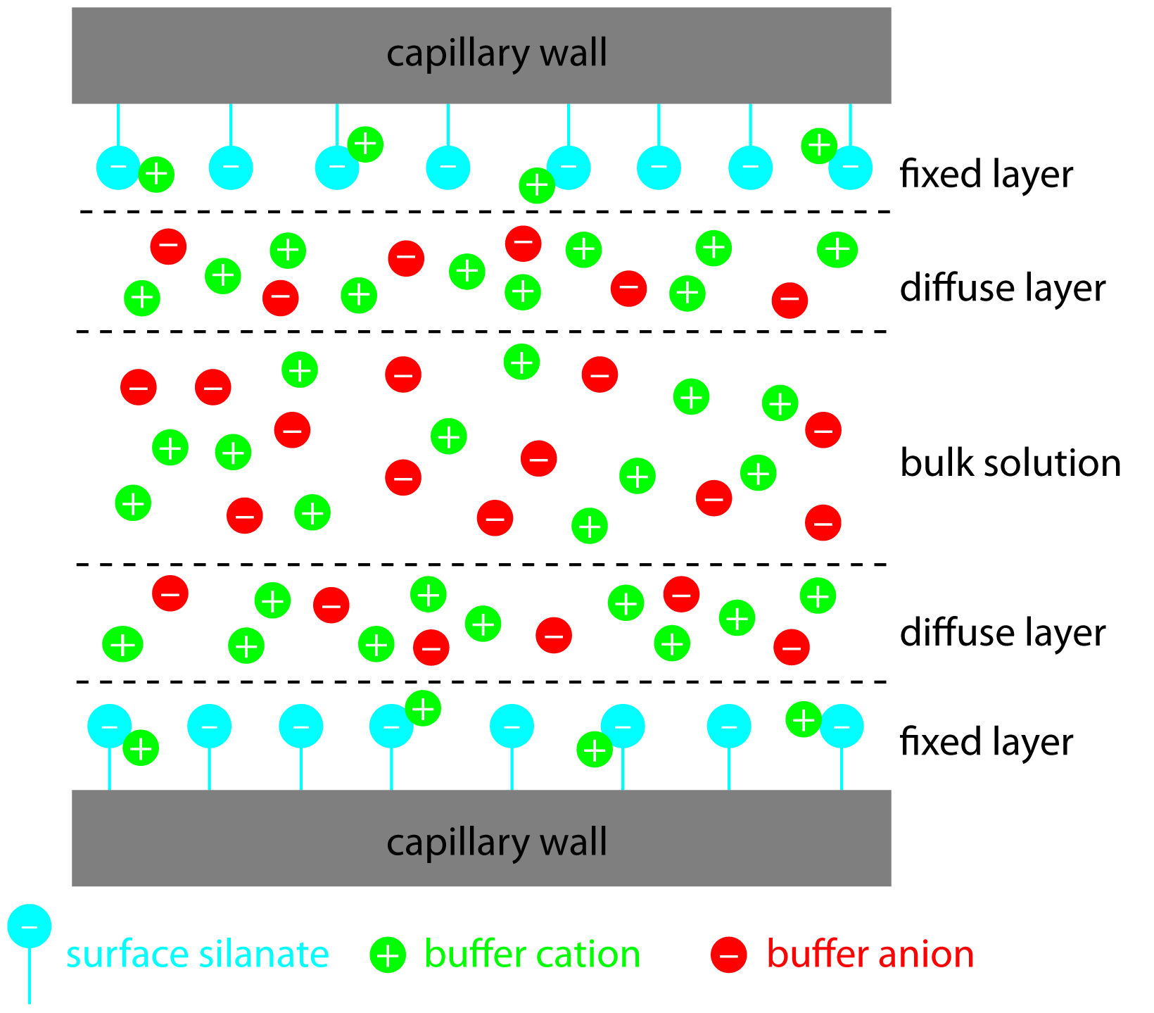
Figure 12.56: Schematic diagram showing the origin of the double layer within a capillary tube. Although the net charge within the capillary is zero, the distribution of charge is not. The walls of the capillary have an excess of negative charge, which decreases across the fixed layer and the diffuse layer, reaching a value of zero in bulk solution.
The rate at which the buffer moves through the capillary, what we call its electroosmotic flow velocity, νeof, is a function of the applied electric field, E, and the buffer’s electroosmotic mobility, μeof.
\[\nu_\ce{eof} = \mu_\ce{eof}E \label{12.36}\]
Electroosmotic mobility is defined as
\[\mu_\ce{eof} = \dfrac{εζ}{4πη} \label{12.37}\]
where
- ε is the buffer dielectric constant,
- ζ is the zeta potential, and
- η is the buffer viscosity.
The zeta potential—the potential of the diffuse layer at a finite distance from the capillary wall—plays an important role in determining the electroosmotic flow velocity. Two factors determine the zeta potential’s value. First, the zeta potential is directly proportional to the charge on the capillary walls, with a greater density of silanate ions corresponding to a larger zeta potential. Below a pH of 2 there are few silanate ions, and the zeta potential and electroosmotic flow velocity are zero. As the pH increases, both the zeta potential and the electroosmotic flow velocity increase. Second, the zeta potential is directly proportional to the thickness of the double layer. Increasing the buffer’s ionic strength provides a higher concentration of cations, decreasing the thickness of the double layer and decreasing the electroosmotic flow.
Zeta Potential
The definition of zeta potential given here is admittedly a bit fuzzy. For a much more technical explanation see Delgado, A. V.; González-Caballero, F.; Hunter, R. J.; Koopal, L. K.; Lyklema, J. “Measurement and Interpretation of Electrokinetic Phenomena,” Pure. Appl. Chem. 2005, 77, 1753–1805. Although this a very technical report, Sections 1.3–1.5 provide a good introduction to the difficulty of defining the zeta potential and measuring its value.
The electroosmotic flow profile is very different from that of a fluid moving under forced pressure. Figure 12.57 compares the electroosmotic flow profile with that the hydrodynamic flow profile in gas chromatography and liquid chromatography. The uniform, flat profile for electroosmosis helps minimize band broadening in capillary electrophoresis, improving separation efficiency.

Figure 12.57: Comparison of hydrodynamic flow and electroosmotic flow. The nearly uniform electroosmotic flow profile means that the electroosmotic flow velocity is nearly constant across the capillary.
Total Mobility
A solute’s total velocity, \(v_{tot}\), as it moves through the capillary is the sum of its electrophoretic velocity and the electroosmotic flow velocity.
\[ν_\ce{tot} =ν_\ce{ep} + ν_\ce{eof}\]
As shown in Figure 12.58, under normal conditions the following general relationships hold true.
\[(ν_\ce{tot})_\ce{cations} > ν_\ce{eof}\]
\[(ν_\ce{tot})_\ce{neutrals} = ν_\ce{eof}\]
\[(ν_\ce{tot})_\ce{anions} < ν_\ce{eof}\]
Cations elute first in an order corresponding to their electrophoretic mobilities, with small, highly charged cations eluting before larger cations of lower charge. Neutral species elute as a single band with an elution rate equal to the electroosmotic flow velocity. Finally, anions are the last components to elute, with smaller, highly charged anions having the longest elution time.
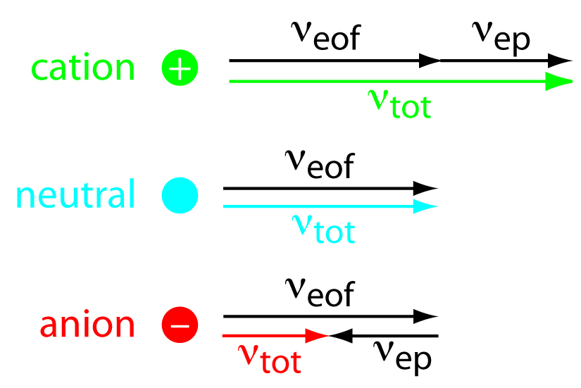
Figure 12.58: Visual explanation for the general elution order in capillary electrophoresis. Each species has the same electroosmotic flow, νeof. Cations elute first because they have a positive electrophoretic velocity, νep. Anions elute last because their negative electrophoretic velocity partially offsets the electroosmotic flow velocity. Neutrals elute with a velocity equal to the electroosmotic flow.
Migration Time
Another way to express a solute’s velocity is to divide the distance it travels by the elapsed time
\[\nu_{tot}=\frac{l}{t_{m}} \label{12.38}\]
where l is the distance between the point of injection and the detector, and tm is the solute’s migration time. To understand the experimental variables affecting migration time, we begin by noting that
\[ν_\ce{tot} = \mu_\ce{tot}E= (\mu_\ce{ep} + \mu_\ce{eof})E\label{12.39}\]
Combining Equations \ref{12.38} and \ref{12.39} and solving for tm leaves us with
\[t_\ce{m} = \dfrac{l}{(\mu_\ce{ep} + \mu_\ce{eof})E}\label{12.40}\]
Finally, the magnitude of the electrical field is
\[E = \dfrac{V}{L}\label{12.41}\]
where V is the applied potential and L is the length of the capillary tube. Finally, substituting Equation \ref{12.41} into Equation \ref{12.40} leaves us with the following equation for a solute’s migration time.
\[t_\ce{m}= \dfrac{lL}{(\mu_\ce{ep} + \mu_\ce{eof})V}\label{12.42}\]
To decrease a solute’s migration time—and shorten the analysis time—we can apply a higher voltage or use a shorter capillary tube. We can also shorten the migration time by increasing the electroosmotic flow, although this decreases resolution.
Efficiency
As we learned in Section 12.2.4, the efficiency of a separation is given by the number of theoretical plates, N. In capillary electrophoresis the number of theoretic plates is
\[N = \dfrac{l^2}{2Dt_\ce{m}} = \dfrac{(\mu_\ce{ep} + \mu_\ce{eof})Vl}{2DL} \label{12.43b}\]
where \(D\) is the solute’s diffusion coefficient.
From Equations \ref{12.10} and \ref{12.11}, we know that the number of theoretical plates for a solute is
\[N = \dfrac{l^2}{\sigma ^2}\]
where l is the distance the solute travels and σ is the standard deviation for the solute’s band broadening. For capillary electrophoresis band broadening is due to longitudinal diffusion and is equivalent to 2Dtm, where tm is the migration time.
From Equation \ref{12.43}, the efficiency of a capillary electrophoretic separation increases with higher voltages. Increasing the electroosmotic flow velocity improves efficiency, but at the expense of resolution. Two additional observations deserve comment. First, solutes with larger electrophoretic mobilities—in the same direction as the electroosmotic flow—have greater efficiencies; thus, smaller, more highly charged cations are not only the first solutes to elute, but do so with greater efficiency. Second, efficiency in capillary electrophoresis is independent of the capillary’s length. Theoretical plate counts of approximately 100,000–200,000 are not unusual.
It is possible to design an electrophoretic experiment so that anions elute before cations—more about this later—in which smaller, more highly charged anions elute with greater efficiencies.
Selectivity
In chromatography we defined the selectivity between two solutes as the ratio of their retention factors (Equation \ref{12.9}). In capillary electrophoresis the analogous expression for selectivity is
\[α = \dfrac{\mu_\textrm{ep,1}}{\mu_\textrm{ep,2}}\]
where μep,1 and μep,2 are the electrophoretic mobilities for the two solutes, chosen such that α ≥ 1. We can often improve selectivity by adjusting the pH of the buffer solution. For example, NH4+ is a weak acid with a pKa of 9.75. At a pH of 9.75 the concentrations of NH4+ and NH3 are equal. Decreasing the pH below 9.75 increases its electrophoretic mobility because a greater fraction of the solute is present as the cation NH4+. On the other hand, raising the pH above 9.75 increases the proportion of the neutral NH3, decreasing its electrophoretic mobility.
Resolution
The resolution between two solutes is
\[R = \dfrac{0.177(\mu_\textrm{ep,1} - \mu_\textrm{ep,2})\sqrt{V}}{\sqrt{D(\mu_\textrm{avg} - \mu_\textrm{eof})}}\label{12.44}\]
where μavg is the average electrophoretic mobility for the two solutes. Increasing the applied voltage and decreasing the electroosmotic flow velocity improves resolution. The latter effect is particularly important. Although increasing electroosmotic flow improves analysis time and efficiency, it decreases resolution.
12.7.2 Instrumentation
The basic instrumentation for capillary electrophoresis is shown in Figure 12.59 and includes a power supply for applying the electric field, anode and cathode compartments containing reservoirs of the buffer solution, a sample vial containing the sample, the capillary tube, and a detector. Each part of the instrument receives further consideration in this section.
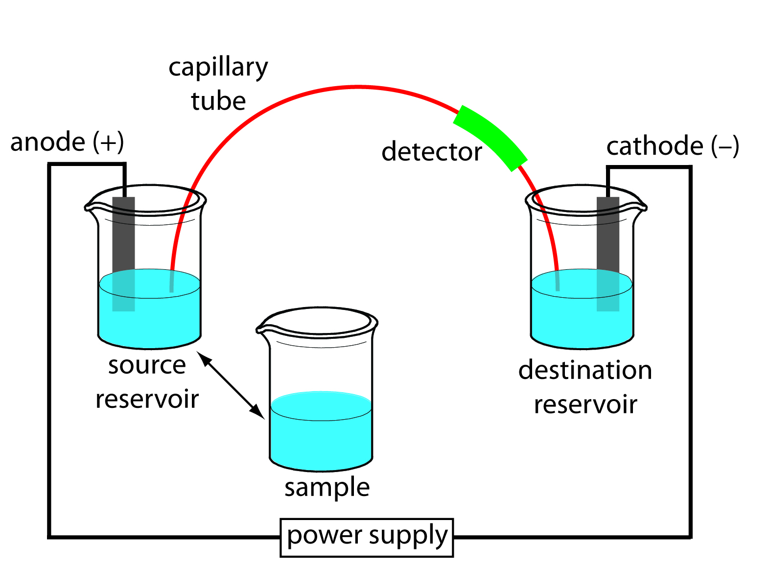
Figure 12.59: Schematic diagram of the basic instrumentation for capillary electrophoresis. The sample and the source reservoir are switched when making injections.
Capillary Tubes
Figure 12.60 shows a cross-section of a typical capillary tube. Most capillary tubes are made from fused silica coated with a 15–35 μm layer of polyimide to give it mechanical strength. The inner diameter is typically 25–75 μm—smaller than the internal diameter of a capillary GC column—with an outer diameter of 200–375 μm.

Figure 12.60: Cross section of a capillary column for capillary electrophoresis. The dimensions shown here are typical and are scaled proportionally.
The capillary column’s narrow opening and the thickness of its walls are important. When an electric field is applied to the buffer solution within the capillary, current flows through the capillary. This current leads to the release of heat—what we call Joule heating. The amount of heat released is proportional to the capillary’s radius and the magnitude of the electrical field. Joule heating is a problem because it changes the buffer solution’s viscosity, with the solution at the center of the capillary being less viscous than that near the capillary walls. Because a solute’s electrophoretic mobility depends on viscosity (Equation \ref{12.35}), solute species in the center of the capillary migrate at a faster rate than those near the capillary walls. The result is an additional source of band broadening that degrades the separation. Capillaries with smaller inner diameters generate less Joule heating, and capillaries with larger outer diameters are more effective at dissipating the heat. Placing the capillary tube inside a thermostated jacket is another method for minimizing the effect of Joule heating; in this case a smaller outer diameter allows for a more rapid dissipation of thermal energy.
Injecting the Sample
There are two commonly used method for injecting a sample into a capillary electrophoresis column: hydrodynamic injection and electrokinetic injection. In both methods the capillary tube is filled with the buffer solution. One end of the capillary tube is placed in the destination reservoir and the other end is placed in the sample vial.
Hydrodynamic injection uses pressure to force a small portion of sample into the capillary tubing. A difference in pressure is applied across the capillary by either pressurizing the sample vial or by applying a vacuum to the destination reservoir. The volume of sample injected, in liters, is given by the following equation
\[V_\ce{inj}= \dfrac{Pd^4πt}{128ηL} \times 10^3\label{12.45}\]
where ∆P is the difference in pressure across the capillary in pascals, d is the capillary’s inner diameter in meters, t is the amount of time that the pressure is applied in seconds, η is the buffer’s viscosity in kg m–1 s–1, and L is the length of the capillary tubing in meters. The factor of 103 changes the units from cubic meters to liters.
For a hydrodynamic injection we move the capillary from the source reservoir to the sample. The anode remains in the source reservoir.
A hydrodynamic injection is also possible by raising the sample vial above the destination reservoir and briefly inserting the filled capillary.
If you want to verify the units in Equation \ref{12.45}, recall from Table 2.2 that 1 Pa is equivalent to 1 kg m-1 s-2.
Example 12.9
In a hydrodynamic injection we apply a pressure difference of 2.5 × 10³ Pa (a ∆P ≈ 0.02 atm) for 2 s to a 75-cm long capillary tube with an internal diameter of 50 μm. Assuming that the buffer’s viscosity is 10–3 kg m–1 s–1, what volume and length of sample did we inject?
Solution
Making appropriate substitutions into equation 12.45 gives the sample’s volume as
\[\begin{align}
V_\ce{inj} &= \mathrm{\dfrac{(2.5×10^3\: kg\: m^{−1}\: s^{−2})(50×10^{−6}\: m)^4(3.14)(2\: s)}{(128)(0.001\: kg\: m^{−1}\: s^{−1})(0.75\:m)} × 10^3\: L/m^3}\\
V_\ce{inj} &= \mathrm{1×10^{−9}\: L = 1\: nL}
\end{align}\]
Because the interior of the capillary is cylindrical, the length of the sample, l, is easy to calculate using the equation for the volume of a cylinder; thus
\[l = \dfrac{V_\ce{inj}}{πr^2} = \mathrm{\dfrac{(1.0×10^{−9}\: L)(10^{−3}\: m^3/L)}{(3.14)(25×10^{−6}\: m)^2} = 5×10^{−4}\: m = 0.5\: mm}\]
Exercise 12.9
Suppose that you need to limit your injection to less than 0.20% of the capillary’s length. Using the information from Example 12.9, what is the maximum injection time for a hydrodynamic injection?
Click here to review your answer to this exercise.
In an electrokinetic injection we place both the capillary and the anode into the sample and briefly apply an potential. The volume of injected sample is the product of the capillary’s cross sectional area and the length of the capillary occupied by the sample. In turn, this length is the product of the solute’s velocity (see equation 12.39) and time; thus
\[l = \dfrac{V_\ce{inj}}{πr^2} = \mathrm{\dfrac{(1.0×10^{−9}\: L)(10^{−3}\: m^3/L)}{(3.14)(25×10^{−6}\: m)^2} = 5×10^{−4}\: m = 0.5\: mm}\]
where
- \(r\) is the capillary’s radius,
- \(L\) is the length of the capillary, and
- \(E′\) is effective electric field in the sample.
An important consequence of equation 12.46 is that an electrokinetic injection is inherently biased toward solutes with larger electrophoretic mobilities. If two solutes have equal concentrations in a sample, we inject a larger volume—and thus more moles—of the solute with the larger μep.
The electric field in the sample is different that the electric field in the rest of the capillary because the sample and the buffer have different ionic compositions. In general, the sample’s ionic strength is smaller, which makes its conductivity smaller. The effective electric field is
\[E′ = E \times \dfrac{κ_\ce{buf}}{κ_\ce{sam}}\]
where κbuf and κsam are the conductivities of the buffer and the sample, respectively.
When an analyte’s concentration is too small to detect reliably, it may be possible to inject it in a manner that increases its concentration in the capillary tube. This method of injection is called stacking. Stacking is accomplished by placing the sample in a solution whose ionic strength is significantly less than that of the buffer in the capillary tube. Because the sample plug has a lower concentration of buffer ions, the effective field strength across the sample plug, E′ is larger than that in the rest of the capillary.
We know from equation 12.34 that electrophoretic velocity is directly proportional to the electrical field. As a result, the cations in the sample plug migrate toward the cathode with a greater velocity, and the anions migrate more slowly—neutral species are unaffected and move with the electroosmotic flow. When the ions reach their respective boundaries between the sample plug and the buffering solution, the electrical field decreases and the electrophoretic velocity of cations decreases and that for anions increases. As shown in Figure 12.61, the result is a stacking of cations and anions into separate, smaller sampling zones. Over time, the buffer within the capillary becomes more homogeneous and the separation proceeds without additional stacking.
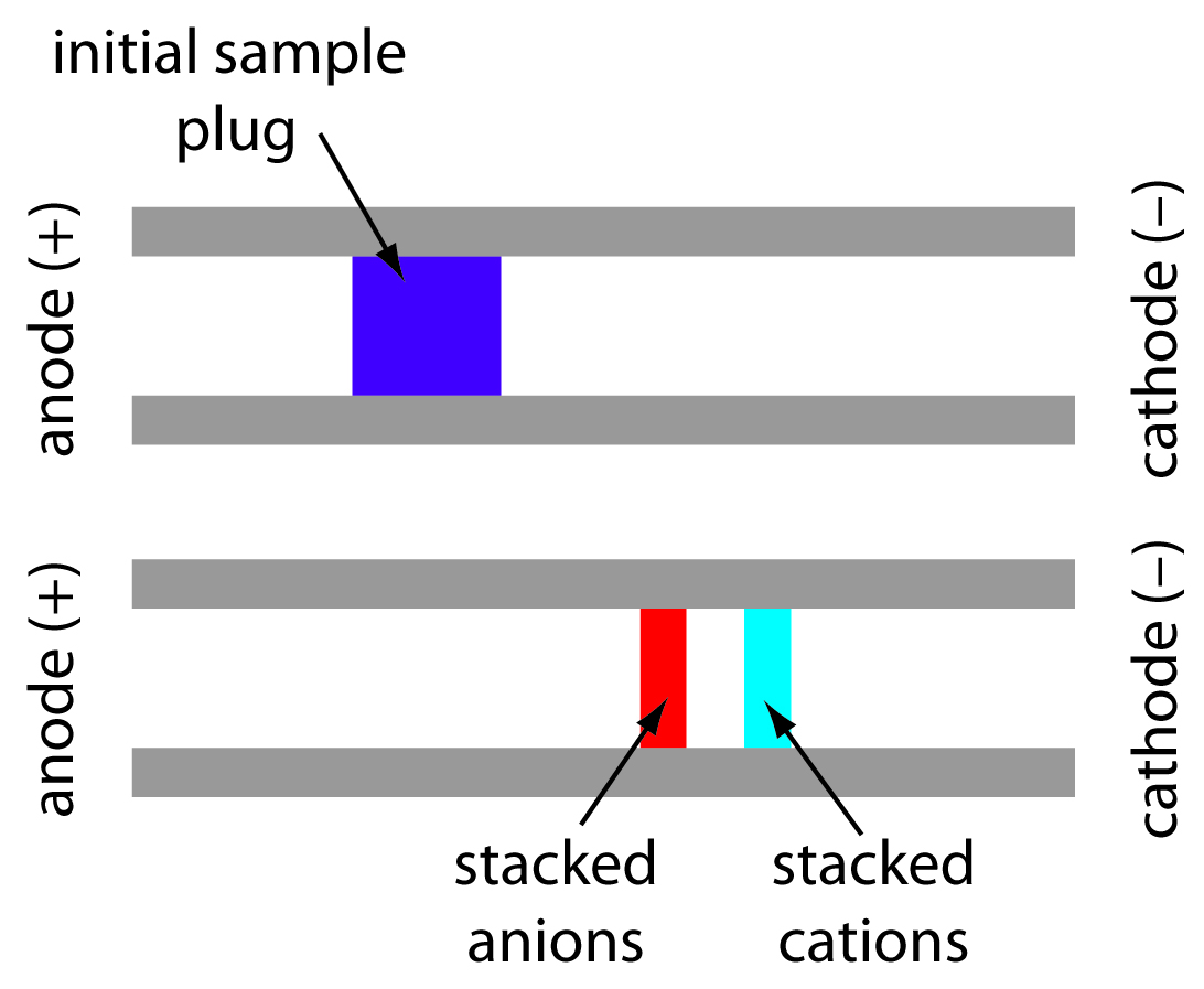
Figure 12.61 The stacking of cations and anions. The top diagram shows the initial sample plug and the bottom diagram shows how the cations and anions become concentrated at opposite sides of the sample plug.
Applying the Electrical Field
Migration in electrophoresis occurs in response to an applied electrical field. The ability to apply a large electrical field is important because higher voltages lead to shorter analysis times (see equation 12.42), more efficient separations (equation 12.43), and better resolution (equation 12.44). Because narrow bored capillary tubes dissipate Joule heating so efficiently, voltages of up to 40 kV are possible.
Because of the high voltages, be sure to follow your instrument’s safety guidelines.
Detectors
Most of the detectors used in HPLC also find use in capillary electrophoresis. Among the more common detectors are those based on the absorption of UV/Vis radiation, fluorescence, conductivity, amperometry, and mass spectrometry. Whenever possible, detection is done “on-column” before the solutes elute from the capillary tube and additional band broadening occurs.
UV/Vis detectors are among the most popular. Because absorbance is directly proportional to path length, the capillary tubing’s small diameter leads to signals that are smaller than those obtained in HPLC. Several approaches have been used to increase the pathlength, including a Z-shaped sample cell and multiple reflections (see Figure 12.62). Detection limits are about 10–7 M.
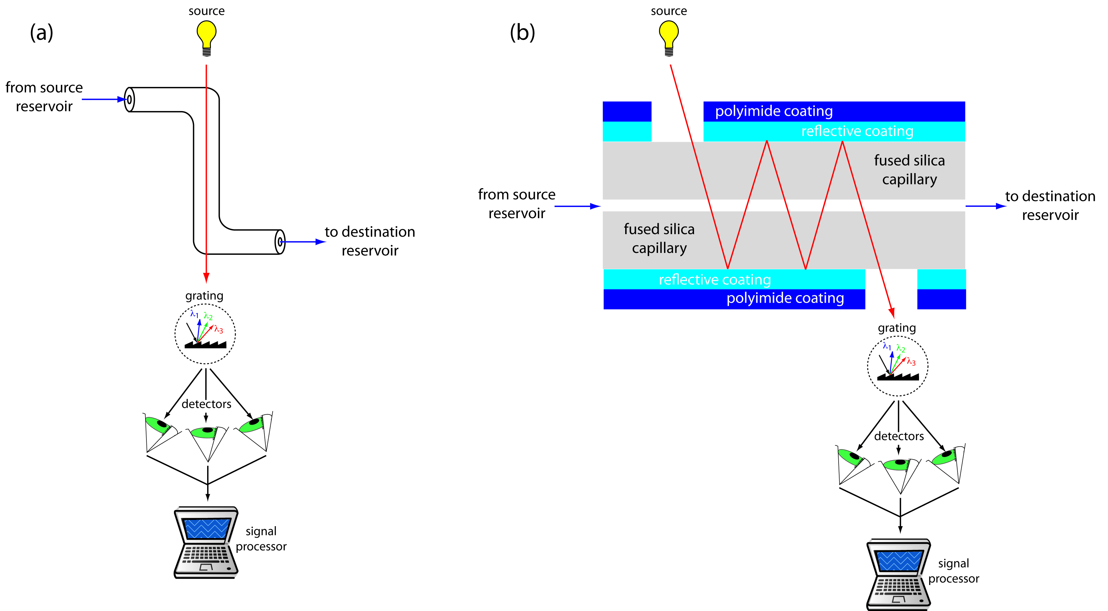
Figure 12.62: Two approaches to on-column detection in capillary electrophoresis using a UV/Vis diode array spectrometer: (a) Z-shaped bend in capillary, and (b) multiple reflections.
Better detection limits are obtained using fluorescence, particularly when using a laser as an excitation source. When using fluorescence detection a small portion of the capillary’s protective coating is removed and the laser beam is focused on the inner portion of the capillary tubing. Emission is measured at an angle of 90o to the laser. Because the laser provides an intense source of radiation that can be focused to a narrow spot, detection limits are as low as 10–16 M.
Solutes that do not absorb UV/Vis radiation or that do not undergo fluorescence can be detected by other detectors. Table 12.10 provides a list of detectors for capillary electrophoresis along with some of their important characteristics.
|
detection limit |
||||
|---|---|---|---|---|
detector |
selectivity universal or analyte must... |
moles injected |
molarity |
on-column detection? |
| UV/Vis absorbance | have a UV/Vis chromophore | 10–13–10–16 | 10–5–10–7 | yes |
| indirect absorbance | universal | 10–12–10–15 | 10–4–10–6 | yes |
| fluorescence | have a favorable quantum yield | 10–15–10–17 | 10–7–10–9 | yes |
| laser fluorescence | have a favorable quantum yield | 10–18–10–20 | 10–13–10–16 | yes |
| mass spectrometer | universal (total ion) selective (single ion) |
10–16–10–17 | 10–8–10–10 | no |
| amperometry | undergo oxidation or reduction | 10–18–10–19 | 10–7–10–10 | no |
| conductivity | universal | 10–15–10–16 | 10–7–10–9 | no |
| radiometric | be radioactive | 10–17–10–19 | 10–10–10–12 | yes |
Source: Baker, D. R. Capillary Electrophoresis, Wiley-Interscience: New York, 1995.
12.7.3 Capillary Electrophoresis Methods
There are several different forms of capillary electrophoresis, each of which has its particular advantages. Four of these methods are briefly described in this section.
Capillary Zone Electrophoresis (CZE)
The simplest form of capillary electrophoresis is capillary zone electrophoresis. In CZE we fill the capillary tube with a buffer solution and, after loading the sample, place the ends of the capillary tube in reservoirs containing additional buffer solution. Usually the end of the capillary containing the sample is the anode and solutes migrate toward the cathode at a velocity determined by their electrophoretic mobility and the electroosmotic flow. Cations elute first, with smaller, more highly charged cations eluting before larger cations with smaller charges. Neutral species elute as a single band. Anions are the last species to elute, with smaller, more negatively charged anions being the last to elute.
We can reverse the direction of electroosmotic flow by adding an alkylammonium salt to the buffer solution. As shown in Figure 12.63, the positively charged end of the alkyl ammonium ions bind to the negatively charged silanate ions on the capillary’s walls. The tail of the alkyl ammonium ion is hydrophobic and associates with the tail of another alkyl ammonium ion. The result is a layer of positive charges that attract anions in the buffer solution. The migration of these solvated anions toward the anode reverses the electroosmotic flow’s direction. The order of elution is exactly opposite of that observed under normal conditions.
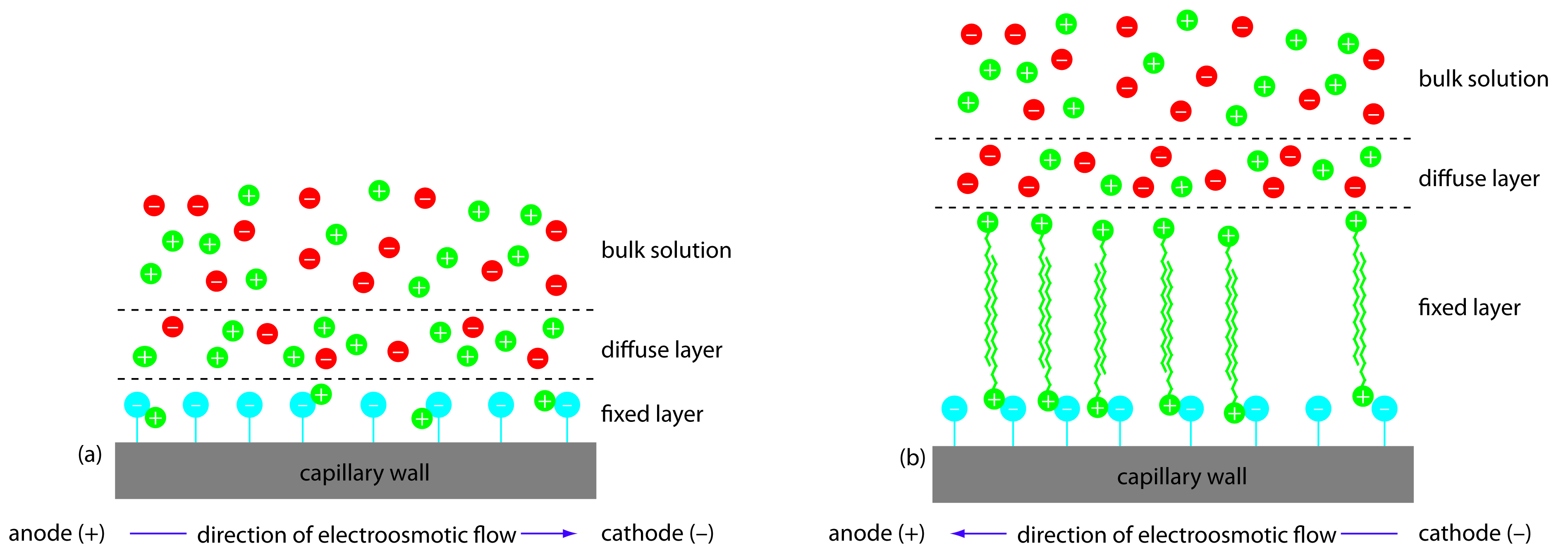
Figure 12.63 Two modes of capillary zone electrophoresis showing (a) normal migration with electroosmotic flow toward the cathode and (b) reversed migration in which the electroosmotic flow is toward the anode.
Coating the capillary’s walls with a nonionic reagent eliminates the electroosmotic flow. In this form of CZE the cations migrate from the anode to the cathode. Anions elute into the source reservoir and neutral species remain stationary.
Capillary zone electrophoresis provides effective separations of charged species, including inorganic anions and cations, organic acids and amines, and large biomolecules such as proteins. For example, CZE has been used to separate a mixture of 36 inorganic and organic ions in less than three minutes.15 A mixture of neutral species, of course, can not be resolved.
Micellar Electrokinetic Capillary Chromatography (MEKC)
One limitation to CZE is its inability to separate neutral species. Micellar electrokinetic capillary chromatography overcomes this limitation by adding a surfactant, such as sodium dodecylsulfate (Figure 12.64a) to the buffer solution. Sodium dodecylsulfate, or SDS, has a long-chain hydrophobic tail and a negatively charged ionic functional group at its head. When the concentration of SDS is sufficiently large a micelle forms. A micelle consists of a spherical agglomeration of 40–100 surfactant molecules in which the hydrocarbon tails point inward and the negatively charged heads point outward (Figure 12.64b).
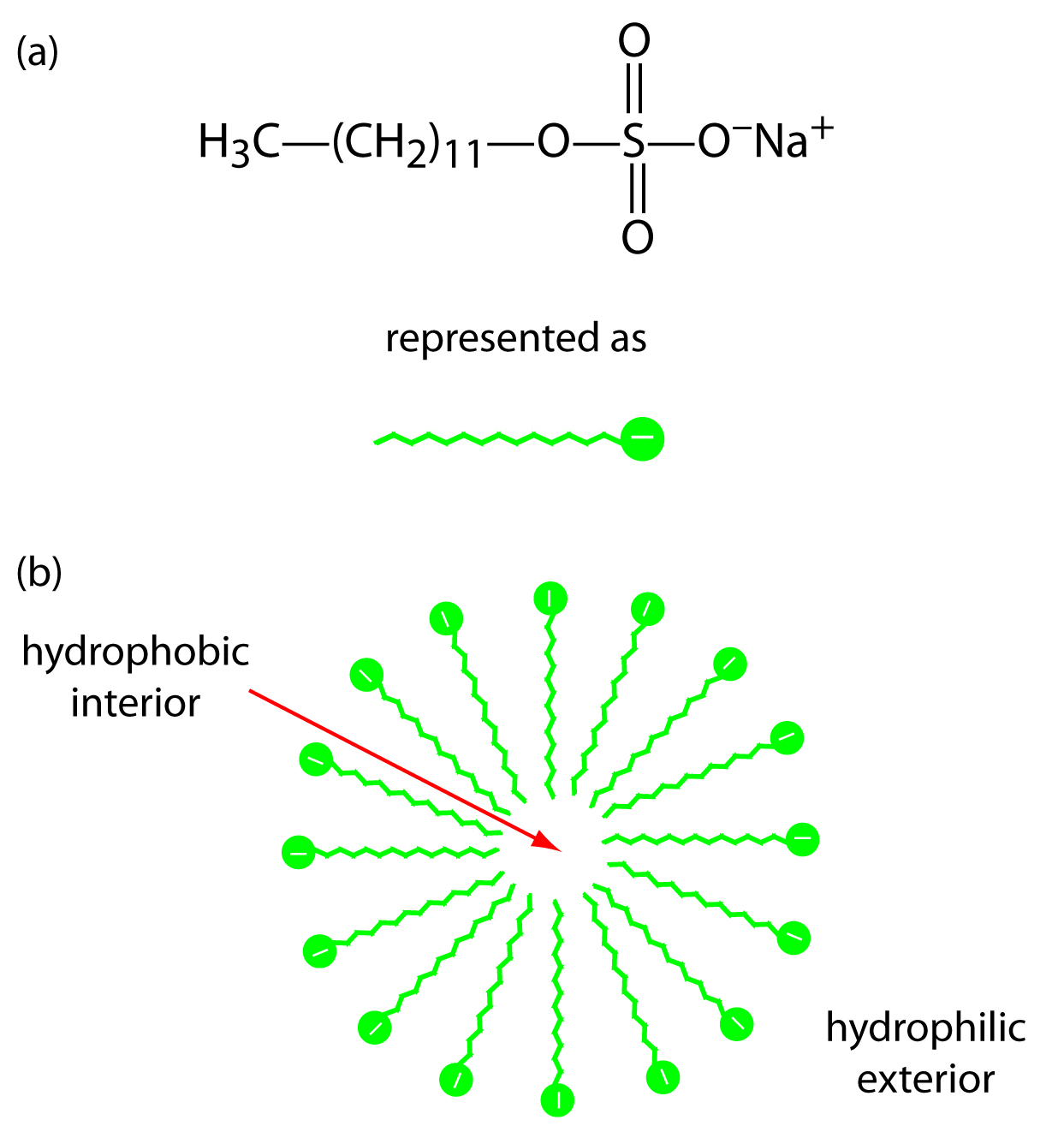
Figure 12.64: (a) Structure of sodium dodecylsulfate and its representation, and (b) cross section through a micelle showing its hydrophobic interior and its hydrophilic exterior.
Because micelles have a negative charge, they migrate toward the cathode with a velocity less than the electroosmotic flow velocity. Neutral species partition themselves between the micelles and the buffer solution in a manner similar to the partitioning of solutes between the two liquid phases in HPLC. Because there is a partitioning between two phases, we include the descriptive term chromatography in the techniques name. Note that in MEKC both phases are mobile.
The elution order for neutral species in MEKC depends on the extent to which each partitions into the micelles. Hydrophilic neutrals are insoluble in the micelle’s hydrophobic inner environment and elute as a single band, as they would in CZE. Neutral solutes that are extremely hydrophobic are completely soluble in the micelle, eluting with the micelles as a single band. Those neutral species that exist in a partition equilibrium between the buffer solution and the micelles elute between the completely hydrophilic and completely hydrophobic neutral species. Those neutral species favoring the buffer solution elute before those favoring the micelles. Micellar electrokinetic chromatography has been used to separate a wide variety of samples, including mixtures of pharmaceutical compounds, vitamins, and explosives.
Capillary Gel Electrophoresis (CGE)
In capillary gel electrophoresis the capillary tubing is filled with a polymeric gel. Because the gel is porous, a solute migrates through the gel with a velocity determined both by its electrophoretic mobility and by its size. The ability to effect a separation using size is helpful when the solutes have similar electrophoretic mobilities. For example, fragments of DNA of varying length have similar charge-to-size ratios, making their separation by CZE difficult. Because the DNA fragments are of different size, a CGE separation is possible.
The capillary used for CGE is usually treated to eliminate electroosmotic flow, preventing the gel’s extrusion from the capillary tubing. Samples are injected electrokinetically because the gel provides too much resistance for hydrodynamic sampling. The primary application of CGE is the separation of large biomolecules, including DNA fragments, proteins, and oligonucleotides.
Capillary Electrochromatography (CEC)
Another approach to separating neutral species is capillary electrochromatography. In CEC the capillary tubing is packed with 1.5–3 μm particles coated with a bonded stationary phase. Neutral species separate based on their ability to partition between the stationary phase and the buffer, which is moving as a result of the electroosmotic flow; Figure 12.65 provides a representative example for the separation of a mixture of hydrocarbons. A CEC separation is similar to the analogous HPLC separation, but without the need for high pressure pumps. Efficiency in CEC is better than in HPLC, and analysis times are shorter.

Figure 12.65: Capillary electrochromatographic separation of a mixture of hydrocarbons in DMSO. The column contains a porous polymer of butyl methacrylate and lauryl acrylate (25%:75% mol:mol) with butane dioldacrylate as a crosslinker. Data provided by Zoe LaPier and Michelle Bushey, Department of Chemistry, Trinity University.
The best way to appreciate the theoretical and practical details discussed in this section is to carefully examine a typical analytical method. Although each method is unique, the following description of the determination of a vitamin B complex by capillary zone electrophoresis or by micellar electrokinetic capillary chromatography provides an instructive example of a typical procedure. The description here is based on Smyth, W. F. Analytical Chemistry of Complex Matrices, Wiley Teubner: Chichester, England, 1996, pp. 154–156.
Representative Method 12.3: Determination of a Vitamin B Complex by CZE or MEKC
Description of Method
The water soluble vitamins B1 (thiamine hydrochloride), B2 (riboflavin), B3 (niacinamide), and B6 (pyridoxine hydrochloride) are determined by CZE using a pH 9 sodium tetraborate-sodium dihydrogen phosphate buffer or by MEKC using the same buffer with the addition of sodium dodecyl sulfate. Detection is by UV absorption at 200 nm. An internal standard of o-ethoxybenzamide is used to standardize the method.
Procedure
Crush a vitamin B complex tablet and place it in a beaker with 20.00 mL of a 50 % v/v methanol solution that is 20 mM in sodium tetraborate and 100.0 ppm in o-ethoxybenzamide. After mixing for 2 min to ensure that the B vitamins are dissolved, pass a 5.00-mL portion through a 0.45-μm filter to remove insoluble binders. Load an approximately 4 nL sample into a capillary column with an inner diameter of a 50 μm. For CZE the capillary column contains a 20 mM pH 9 sodium tetraborate-sodium dihydrogen phosphate buffer. For MEKC the buffer is also 150 mM in sodium dodecyl sulfate. Apply a 40 kV/m electrical field to effect both the CZE and MEKC separations.
Questions
1. Methanol, which elutes at 4.69 min, is included as a neutral species to indicate the electroosmotic flow. When using standard solutions of each vitamin, CZE peaks are found at 3.41 min, 4.69 min, 6.31 min, and 8.31 min. Examine the structures and pKa information in Figure 12.66 and identify the order in which the four B vitamins elute.
Vitamin B1 is a cation and elutes before the neutral species methanol; thus it is the compound that elutes at 3.41 min. Vitamin B3 is a neutral species and elutes with methanol at 4.69 min. The remaining two B vitamins are weak acids that partially ionize to weak base anions in the pH 9 buffer. Of the two, vitamin B6 is the stronger acid (a pKa of 9.0 versus a pKa of 9.7) and is present to a greater extent in its anionic form. Vitamin B6, therefore, is the last of the vitamins to elute.
2. The order of elution when using MEKC is vitamin B3 (5.58 min), vitamin B6 (6.59 min), vitamin B2 (8.81 min), and vitamin B1 (11.21 min). What conclusions can you make about the solubility of the B vitamins in the sodium dodecylsulfate micelles? The micelles elute at 17.7 min.
The elution time for vitamin B1 shows the greatest change, increasing from 3.41 min to 11.21 minutes. Clearly vitamin B1 has the greatest solubility in the micelles. Vitamin B2 and vitamin B3 have a more limited solubility in the micelles, showing only slightly longer elution times in the presence of the micelles. Interestingly, the elution time for vitamin B6 decreases in the presence of the micelles.
3. For quantitative work an internal standard of o-ethoxybenzamide is added to all samples and standards. Why is an internal standard necessary?
Although the method of injection is not specified, neither a hydrodynamic injection nor an electrokinetic injection is particularly reproducible. The use of an internal standard compensates for this limitation.
(You can read more about the use of internal standards in capillary electrophoresis in the following paper: Altria, K. D. “Improved Performance in Capillary Electrophoresis Using Internal Standards,” LC.GC Europe, September 2002.)
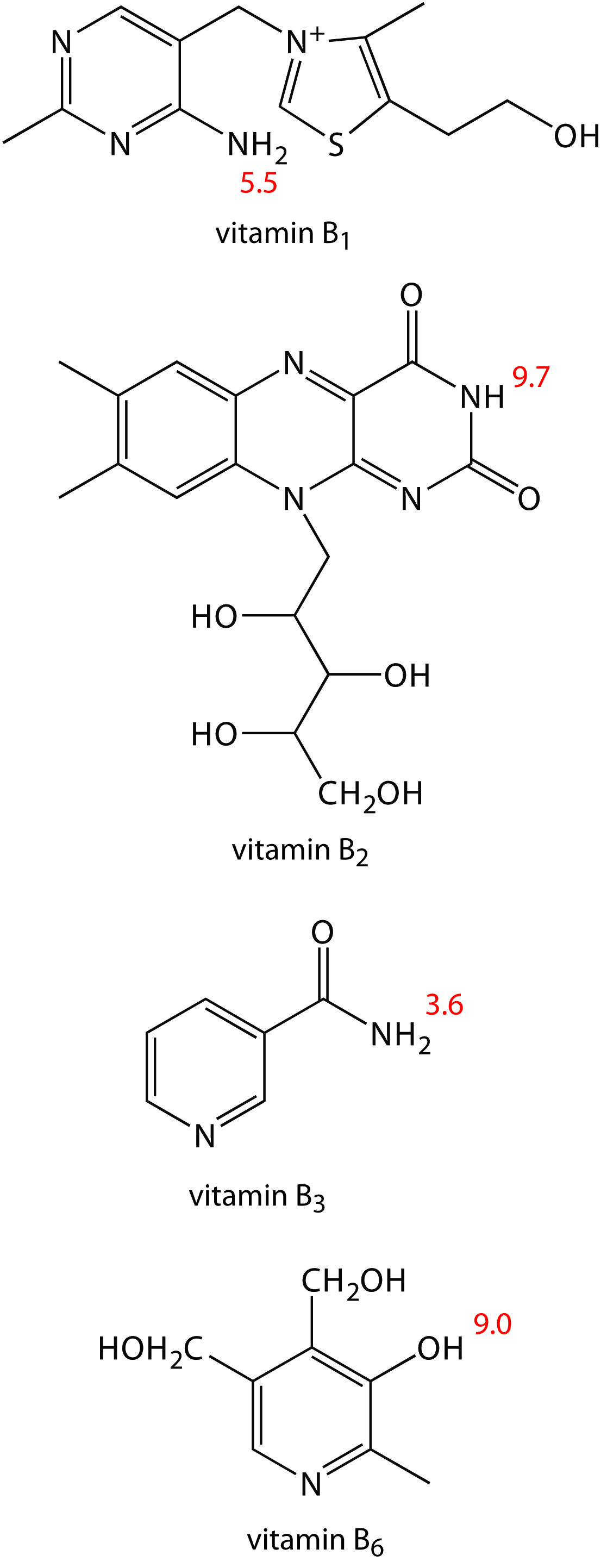
Figure 12.66: Structures of the four water soluble B vitamins in their predominate forms at a pH of 9; pKa values are shown in red.
12.7.4 Evaluation
When compared to GC and HPLC, capillary electrophoresis provides similar levels of accuracy, precision, and sensitivity, and a comparable degree of selectivity. The amount of material injected into a capillary electrophoretic column is significantly smaller than that for GC and HPLC—typically 1 nL versus 0.1 μL for capillary GC and 1–100 μL for HPLC. Detection limits for capillary electrophoresis, however, are 100–1000 times poorer than that for GC and HPLC. The most significant advantages of capillary electrophoresis are improvements in separation efficiency, time, and cost. Capillary electrophoretic columns contain substantially more theoretical plates (≈106 plates/m) than that found in HPLC (≈105 plates/m) and capillary GC columns (≈103 plates/m), providing unparalleled resolution and peak capacity. Separations in capillary electrophoresis are fast and efficient. Furthermore, the capillary column’s small volume means that a capillary electrophoresis separation requires only a few microliters of buffer solution, compared to 20–30 mL of mobile phase for a typical HPLC separation.
Note
See Section 12.4.8 for an evaluation of gas chromatography, and Section 12.5.6 for an evaluation of high-performance liquid chromatography.