
10.6: Photoluminescence Spectroscopy
- Page ID
- 5613

\( \newcommand{\vecs}[1]{\overset { \scriptstyle \rightharpoonup} {\mathbf{#1}} } \)
\( \newcommand{\vecd}[1]{\overset{-\!-\!\rightharpoonup}{\vphantom{a}\smash {#1}}} \)
\( \newcommand{\id}{\mathrm{id}}\) \( \newcommand{\Span}{\mathrm{span}}\)
( \newcommand{\kernel}{\mathrm{null}\,}\) \( \newcommand{\range}{\mathrm{range}\,}\)
\( \newcommand{\RealPart}{\mathrm{Re}}\) \( \newcommand{\ImaginaryPart}{\mathrm{Im}}\)
\( \newcommand{\Argument}{\mathrm{Arg}}\) \( \newcommand{\norm}[1]{\| #1 \|}\)
\( \newcommand{\inner}[2]{\langle #1, #2 \rangle}\)
\( \newcommand{\Span}{\mathrm{span}}\)
\( \newcommand{\id}{\mathrm{id}}\)
\( \newcommand{\Span}{\mathrm{span}}\)
\( \newcommand{\kernel}{\mathrm{null}\,}\)
\( \newcommand{\range}{\mathrm{range}\,}\)
\( \newcommand{\RealPart}{\mathrm{Re}}\)
\( \newcommand{\ImaginaryPart}{\mathrm{Im}}\)
\( \newcommand{\Argument}{\mathrm{Arg}}\)
\( \newcommand{\norm}[1]{\| #1 \|}\)
\( \newcommand{\inner}[2]{\langle #1, #2 \rangle}\)
\( \newcommand{\Span}{\mathrm{span}}\) \( \newcommand{\AA}{\unicode[.8,0]{x212B}}\)
\( \newcommand{\vectorA}[1]{\vec{#1}} % arrow\)
\( \newcommand{\vectorAt}[1]{\vec{\text{#1}}} % arrow\)
\( \newcommand{\vectorB}[1]{\overset { \scriptstyle \rightharpoonup} {\mathbf{#1}} } \)
\( \newcommand{\vectorC}[1]{\textbf{#1}} \)
\( \newcommand{\vectorD}[1]{\overrightarrow{#1}} \)
\( \newcommand{\vectorDt}[1]{\overrightarrow{\text{#1}}} \)
\( \newcommand{\vectE}[1]{\overset{-\!-\!\rightharpoonup}{\vphantom{a}\smash{\mathbf {#1}}}} \)
\( \newcommand{\vecs}[1]{\overset { \scriptstyle \rightharpoonup} {\mathbf{#1}} } \)
\( \newcommand{\vecd}[1]{\overset{-\!-\!\rightharpoonup}{\vphantom{a}\smash {#1}}} \)
\(\newcommand{\avec}{\mathbf a}\) \(\newcommand{\bvec}{\mathbf b}\) \(\newcommand{\cvec}{\mathbf c}\) \(\newcommand{\dvec}{\mathbf d}\) \(\newcommand{\dtil}{\widetilde{\mathbf d}}\) \(\newcommand{\evec}{\mathbf e}\) \(\newcommand{\fvec}{\mathbf f}\) \(\newcommand{\nvec}{\mathbf n}\) \(\newcommand{\pvec}{\mathbf p}\) \(\newcommand{\qvec}{\mathbf q}\) \(\newcommand{\svec}{\mathbf s}\) \(\newcommand{\tvec}{\mathbf t}\) \(\newcommand{\uvec}{\mathbf u}\) \(\newcommand{\vvec}{\mathbf v}\) \(\newcommand{\wvec}{\mathbf w}\) \(\newcommand{\xvec}{\mathbf x}\) \(\newcommand{\yvec}{\mathbf y}\) \(\newcommand{\zvec}{\mathbf z}\) \(\newcommand{\rvec}{\mathbf r}\) \(\newcommand{\mvec}{\mathbf m}\) \(\newcommand{\zerovec}{\mathbf 0}\) \(\newcommand{\onevec}{\mathbf 1}\) \(\newcommand{\real}{\mathbb R}\) \(\newcommand{\twovec}[2]{\left[\begin{array}{r}#1 \\ #2 \end{array}\right]}\) \(\newcommand{\ctwovec}[2]{\left[\begin{array}{c}#1 \\ #2 \end{array}\right]}\) \(\newcommand{\threevec}[3]{\left[\begin{array}{r}#1 \\ #2 \\ #3 \end{array}\right]}\) \(\newcommand{\cthreevec}[3]{\left[\begin{array}{c}#1 \\ #2 \\ #3 \end{array}\right]}\) \(\newcommand{\fourvec}[4]{\left[\begin{array}{r}#1 \\ #2 \\ #3 \\ #4 \end{array}\right]}\) \(\newcommand{\cfourvec}[4]{\left[\begin{array}{c}#1 \\ #2 \\ #3 \\ #4 \end{array}\right]}\) \(\newcommand{\fivevec}[5]{\left[\begin{array}{r}#1 \\ #2 \\ #3 \\ #4 \\ #5 \\ \end{array}\right]}\) \(\newcommand{\cfivevec}[5]{\left[\begin{array}{c}#1 \\ #2 \\ #3 \\ #4 \\ #5 \\ \end{array}\right]}\) \(\newcommand{\mattwo}[4]{\left[\begin{array}{rr}#1 \amp #2 \\ #3 \amp #4 \\ \end{array}\right]}\) \(\newcommand{\laspan}[1]{\text{Span}\{#1\}}\) \(\newcommand{\bcal}{\cal B}\) \(\newcommand{\ccal}{\cal C}\) \(\newcommand{\scal}{\cal S}\) \(\newcommand{\wcal}{\cal W}\) \(\newcommand{\ecal}{\cal E}\) \(\newcommand{\coords}[2]{\left\{#1\right\}_{#2}}\) \(\newcommand{\gray}[1]{\color{gray}{#1}}\) \(\newcommand{\lgray}[1]{\color{lightgray}{#1}}\) \(\newcommand{\rank}{\operatorname{rank}}\) \(\newcommand{\row}{\text{Row}}\) \(\newcommand{\col}{\text{Col}}\) \(\renewcommand{\row}{\text{Row}}\) \(\newcommand{\nul}{\text{Nul}}\) \(\newcommand{\var}{\text{Var}}\) \(\newcommand{\corr}{\text{corr}}\) \(\newcommand{\len}[1]{\left|#1\right|}\) \(\newcommand{\bbar}{\overline{\bvec}}\) \(\newcommand{\bhat}{\widehat{\bvec}}\) \(\newcommand{\bperp}{\bvec^\perp}\) \(\newcommand{\xhat}{\widehat{\xvec}}\) \(\newcommand{\vhat}{\widehat{\vvec}}\) \(\newcommand{\uhat}{\widehat{\uvec}}\) \(\newcommand{\what}{\widehat{\wvec}}\) \(\newcommand{\Sighat}{\widehat{\Sigma}}\) \(\newcommand{\lt}{<}\) \(\newcommand{\gt}{>}\) \(\newcommand{\amp}{&}\) \(\definecolor{fillinmathshade}{gray}{0.9}\)Photoluminescence is divided into two categories: fluorescence and phosphorescence. A pair of electrons occupying the same electronic ground state have opposite spins and are said to be in a singlet spin state (Figure 10.47a). When an analyte absorbs an ultraviolet or visible photon, one of its valence electrons moves from the ground state to an excited state with a conservation of the electron’s spin (Figure 10.47b). Emission of a photon from the singlet excited state to the singlet ground state—or between any two energy levels with the same spin—is called fluorescence. The probability of fluorescence is very high and the average lifetime of an electron in the excited state is only 10–5–10–8 s. Fluorescence, therefore, decays rapidly once the source of excitation is removed.
In some cases an electron in a singlet excited state is transformed to a triplet excited state (Figure 10.47c) in which its spin is no longer paired with the ground state. Emission between a triplet excited state and a singlet ground state—or between any two energy levels that differ in their respective spin states–is called phosphorescence. Because the average lifetime for phosphorescence ranges from 10–4–104 s, phosphorescence may continue for some time after removing the excitation source.
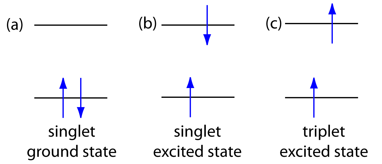
Figure 10.47 Electron configurations for (a) a singlet ground state; (b) a singlet excited state; and (c) a triplet excited state.
The use of molecular fluorescence for qualitative analysis and semi-quantitative analysis can be traced to the early to mid 1800s, with more accurate quantitative methods appearing in the 1920s. Instrumentation for fluorescence spectroscopy using a filter or a monochromator for wavelength selection appeared in, respectively, the 1930s and 1950s. Although the discovery of phosphorescence preceded that of fluorescence by almost 200 years, qualitative and quantitative applications of molecular phosphorescence did not receive much attention until after the development of fluorescence instrumentation.
10.6.1 Fluorescence and Phosphorescence Spectra
To appreciate the origin of fluorescence and phosphorescence we must consider what happens to a molecule following the absorption of a photon. Let’s assume that the molecule initially occupies the lowest vibrational energy level of its electronic ground state, which is a singlet state labeled S0 in Figure 10.48. Absorption of a photon excites the molecule to one of several vibrational energy levels in the first excited electronic state, S1, or the second electronic excited state, S2, both of which are singlet states. Relaxation to the ground state occurs by a number of mechanisms, some involving the emission of photons and others occurring without emitting photons. These relaxation mechanisms are shown in Figure 10.48. The most likely relaxation pathway is the one with the shortest lifetime for the excited state.
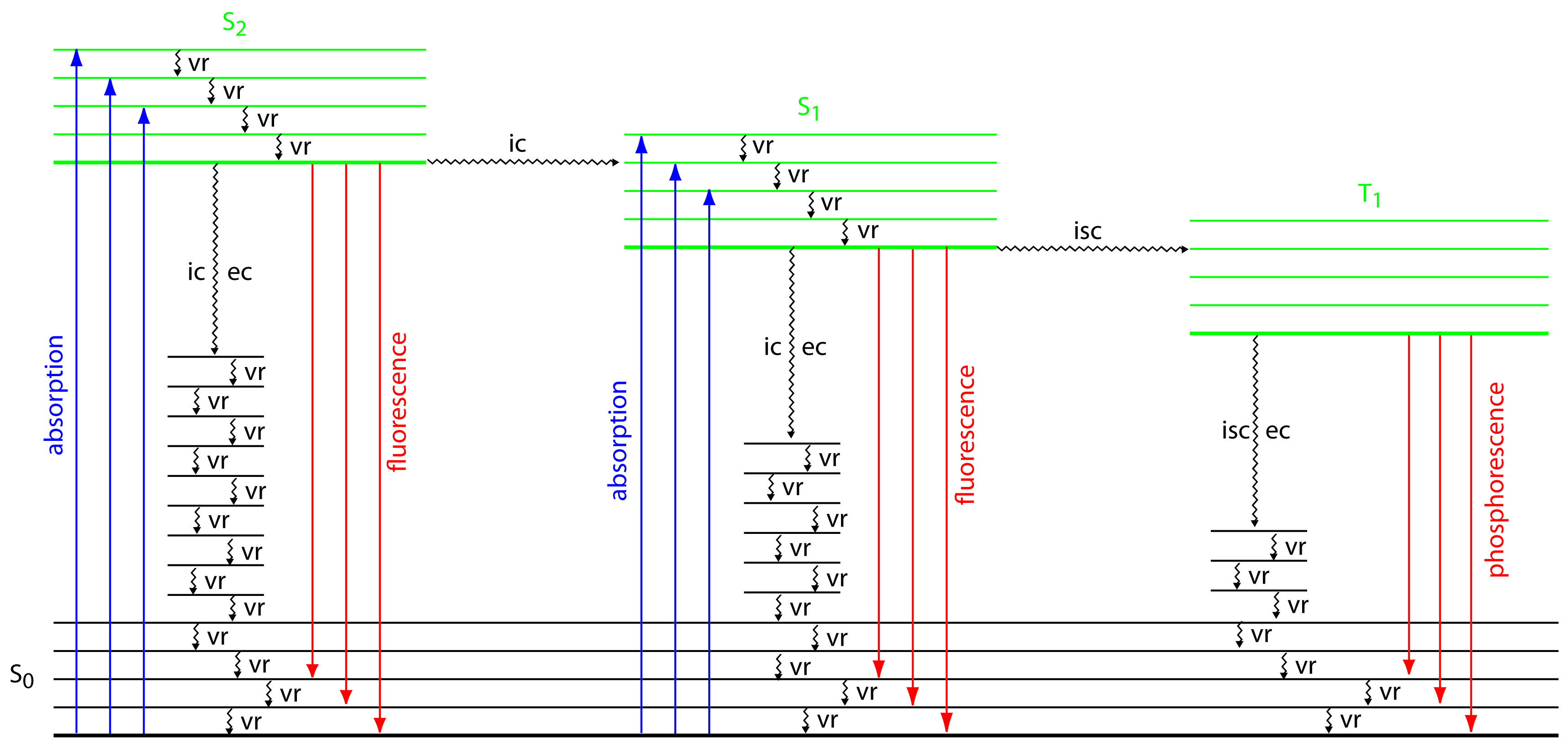
Figure 10.48 Energy level diagram for a molecule showing pathways for the deactivation of an excited state: vr is vibrational relaxation; ic is internal conversion; ec is external conversion; and isc is an intersystem crossing. The lowest vibrational energy for each electronic state is indicated by the thicker line. The electronic ground state is shown in black and the three electronic excited states are shown in green. The absorption, fluorescence, and phosphorescence of photons also are shown.
Radiationless Deactivation
When a molecule relaxes without emitting a photon we call the process radiationless deactivation. One example of radiationless deactivation is vibrational relaxation, in which a molecule in an excited vibrational energy level loses energy by moving to a lower vibrational energy level in the same electronic state. Vibrational relaxation is very rapid, with an average lifetime of <10–12 s. Because vibrational relaxation is so efficient, a molecule in one of its excited state’s higher vibrational energy levels quickly returns to the excited state’s lowest vibrational energy level.
Another form of radiationless deactivation is an internal conversion in which a molecule in the ground vibrational level of an excited state passes directly into a higher vibrational energy level of a lower energy electronic state of the same spin state. By a combination of internal conversions and vibrational relaxations, a molecule in an excited electronic state may return to the ground electronic state without emitting a photon. A related form of radiationless deactivation is an external conversion in which excess energy is transferred to the solvent or to another component of the sample’s matrix.
A final form of radiationless deactivation is an intersystem crossing in which a molecule in the ground vibrational energy level of an excited electronic state passes into a higher vibrational energy level of a lower energy electronic state with a different spin state. For example, an intersystem crossing is shown in Figure 10.48 between a singlet excited state, S1, and a triplet excited state, T1.
Note
Let’s use Figure 10.48 to illustrate how a molecule can relax back to its ground state without emitting a photon. Suppose our molecule is in the highest vibrational energy level of the second electronic excited state. After a series of vibrational relaxations brings the molecule to the lowest vibrational energy level of S2, it undergoes an internal conversion into a higher vibrational energy level of the first excited electronic state. Vibrational relaxations bring the molecule to the lowest vibrational energy level of S1. Following an internal conversion into a higher vibrational energy level of the ground state, the molecule continues to undergo vibrational relaxation until it reaches the lowest vibrational energy level of S0.
Relaxation by Fluorescence
Fluorescence occurs when a molecule in an excited state’s lowest vibrational energy level returns to a lower energy electronic state by emitting a photon. Because molecules return to their ground state by the fastest mechanism, fluorescence is observed only if it is a more efficient means of relaxation than a combination of internal conversions and vibrational relaxations.
A quantitative expression of fluorescence efficiency is the fluorescent quantum yield, Φf, which is the fraction of excited state molecules returning to the ground state by fluorescence. Fluorescent quantum yields range from 1, when every molecule in an excited state undergoes fluorescence, to 0 when fluorescence does not occur.
The intensity of fluorescence, If, is proportional to the amount of radiation absorbed by the sample, P0 – PT, and the fluorescent quantum yield
\[I_\ce{f} = kΦ_\ce{f}(P_0 − P_\ce{T})\tag{10.25}\]
where k is a constant accounting for the efficiency of collecting and detecting the fluorescent emission. From Beer’s law we know that
\[\dfrac{P_\ce{T}}{P_0} = 10^{−εbC}\tag{10.26}\]
where C is the concentration of the fluorescing species. Solving equation 10.26 for PT and substituting into equation 10.25 gives, after simplifying
\[I_\ce{f} = kΦ_\ce{f}P_0(1 − 10^{−εbC})\tag{10.27}\]
When εbC< 0.01, which often is the case when concentration is small, equation 10.27 simplifies to
\[I_\ce{f} = 2.303kΦ_\ce{f}εbCP_0 = k′P_0\tag{10.28}\]
where k′ is a collection of constants. The intensity of fluorescent emission, therefore, increases with an increase in the quantum efficiency, the sourcefs incident power, and the molar absorptivity and the concentration of the fluorescing species.
Fluorescence is generally observed when the molecule’s lowest energy absorption is a π → π* transition, although some n → π* transitions show weak fluorescence. Most unsubstituted, nonheterocyclic aromatic compounds have favorable fluorescence quantum yields, although substitutions on the aromatic ring can significantly effect Φf. For example, the presence of an electron-withdrawing group, such as –NO2, decreases Φf, while adding an electron-donating group, such as –OH, increases Φf. Fluorescence also increases for aromatic ring systems and for aromatic molecules with rigid planar structures. Figure 10.49 shows the fluorescence of quinine under a UV lamp.

Figure 10.49 Tonic water, which contains quinine, is fluorescent when placed under a UV lamp. Source: Splarka (commons.wikipedia.org).
A molecule’s fluorescent quantum yield is also influenced by external variables, such as temperature and solvent. Increasing the temperature generally decreases Φf because more frequent collisions between the molecule and the solvent increases external conversion. A decrease in the solvent’s viscosity decreases Φf for similar reasons. For an analyte with acidic or basic functional groups, a change in pH may change the analyte’s structure and its fluorescent properties.
As shown in Figure 10.48, fluorescence may return the molecule to any of several vibrational energy levels in the ground electronic state. Fluorescence, therefore, occurs over a range of wavelengths. Because the change in energy for fluorescent emission is generally less than that for absorption, a molecule’s fluorescence spectrum is shifted to higher wavelengths than its absorption spectrum.
Relaxation by Phosphorescence
A molecule in a triplet electronic excited state’s lowest vibrational energy level normally relaxes to the ground state by an intersystem crossing to a singlet state or by an external conversion. Phosphorescence occurs when the molecule relaxes by emitting a photon. As shown in Figure 10.48, phosphorescence occurs over a range of wavelengths, all of which are at lower energies than the molecule’s absorption band. The intensity of phosphorescence, Ip, is given by an equation similar to equation 10.28 for fluorescence
\[I_\ce{p} = 2.303kΦ_\ce{p}εbCP_0 = k′P_0\tag{10.29}\]
where Φp is the phosphorescent quantum yield.
Phosphorescence is most favorable for molecules with n → π* transitions, which have a higher probability for an intersystem crossing than π → π* transitions. For example, phosphorescence is observed with aromatic molecules containing carbonyl groups or heteroatoms. Aromatic compounds containing halide atoms also have a higher efficiency for phosphorescence. In general, an increase in phosphorescence corresponds to a decrease in fluorescence.
Because the average lifetime for phosphorescence is very long, ranging from 10–4–104 s, the phosphorescent quantum yield is usually quite small. An improvement in Φp is realized by decreasing the efficiency of external conversion. This may be accomplished in several ways, including lowering the temperature, using a more viscous solvent, depositing the sample on a solid substrate, or trapping the molecule in solution. Figure 10.50 shows an example of phosphorescence.
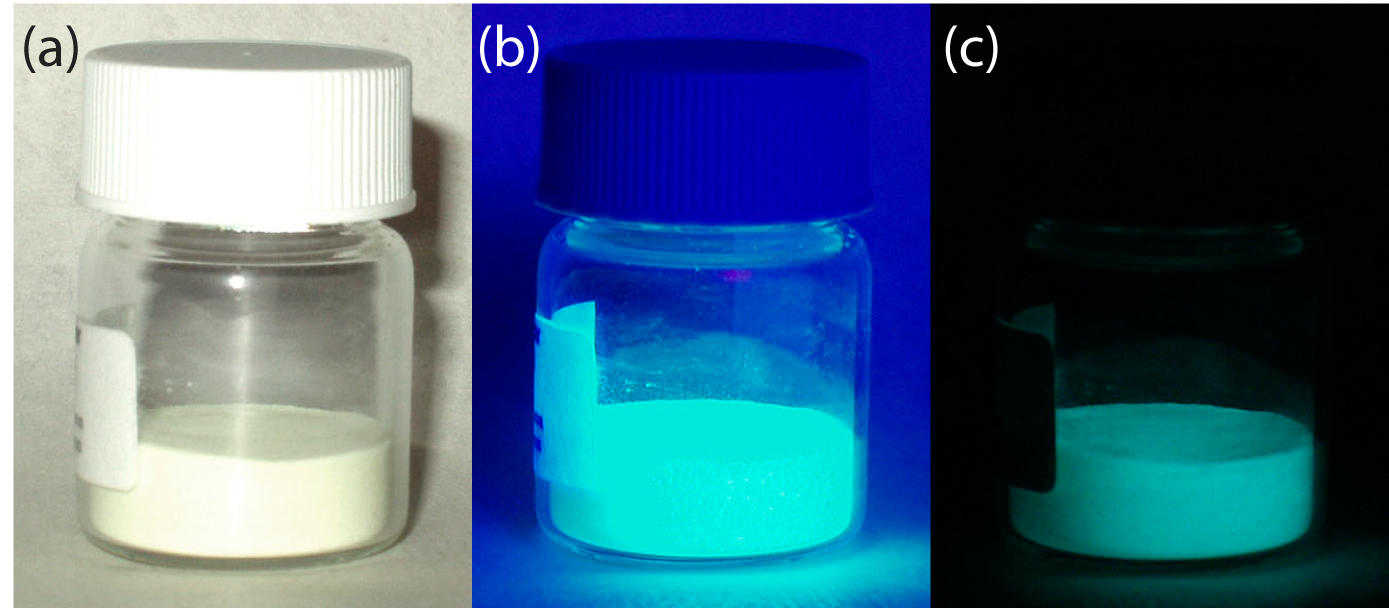
Figure 10.50 An europium doped strontium silicate-aluminum oxide powder under (a) natural light, (b) a long-wave UV lamp, and (c) in total darkness. The photo taken in total darkness shows the phosphorescent emission. Source: modified from Splarka (commons.wikipedia.org).
Excitation versus Emission Spectra
Photoluminescence spectra are recorded by measuring the intensity of emitted radiation as a function of either the excitation wavelength or the emission wavelength. An excitation spectrum is obtained by monitoring emission at a fixed wavelength while varying the excitation wavelength. When corrected for variations in the source’s intensity and the detector’s response, a sample’s excitation spectrum is nearly identical to its absorbance spectrum. The excitation spectrum provides a convenient means for selecting the best excitation wavelength for a quantitative or qualitative analysis.
In an emission spectrum a fixed wavelength is used to excite the sample and the intensity of emitted radiation is monitored as function of wavelength. Although a molecule has only a single excitation spectrum, it has two emission spectra, one for fluorescence and one for phosphorescence. Figure 10.51 shows the UV absorption spectrum and the UV fluorescence emission spectrum for tyrosine.

Figure 10.51 Absorbance spectrum and fluorescence emission spectrum for tyrosine in a pH 7, 0.1 M phosphate buffer. The emission spectrum uses an excitation wavelength of 260 nm. Source: modified from Mark Somoza (commons.wikipedia.org).
10.6.2 Instrumentation
The basic instrumental needs for monitoring fluorescence and phosphorescence—a source of radiation, a means of selecting a narrow band of radiation, and a detector—are the same as those for absorption spectroscopy. The unique demands of both techniques, however, require some modifications to the instrument designs seen earlier in Figure 10.25 (filter photometer), Figure 10.26 (single-beam spectrophotometer), Figure 10.27 (double-beam spectrophotometer), and Figure 10.28 (diode array spectrometer). The most important difference is the detector cannot be placed directly across from the source. Figure 10.52 shows why this is the case. If we place the detector along the source’s axis it will receive both the transmitted source radiation, PT, and the fluorescent, If, or phosphorescent, Ip, radiation. Instead, we rotate the director and place it at 90o to the source.
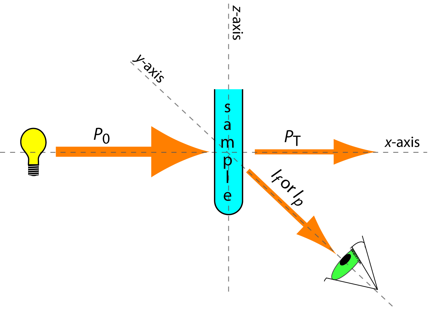
Figure 10.52 Schematic diagram showing the orientation of the source and the detector when measuring fluorescence and phosphorescence. Contrast this to Figure 10.21, which shows the orientation for absorption spectroscopy.
Instruments for Measuring Fluorescence
Figure 10.53 shows the basic design of an instrument for measuring fluorescence, which includes two wavelength selectors, one for selecting an excitation wavelength from the source and one for selecting the emission wavelength from the sample. In a fluorimeter the excitation and emission wavelengths are selected using absorption or interference filters. The excitation source for a fluorimeter is usually a low-pressure Hg vapor lamp that provides intense emission lines distributed throughout the ultraviolet and visible region (254, 312, 365, 405, 436, 546, 577, 691, and 773 nm). When a monochromator is used to select the excitation and emission wavelengths, the instrument is called a spectrofluorimeter. With a monochromator the excitation source is usually high-pressure Xe arc lamp, which has a continuous emission spectrum. Either instrumental design is appropriate for quantitative work, although only a spectrofluorimeter can be used to record an excitation or emission spectrum.
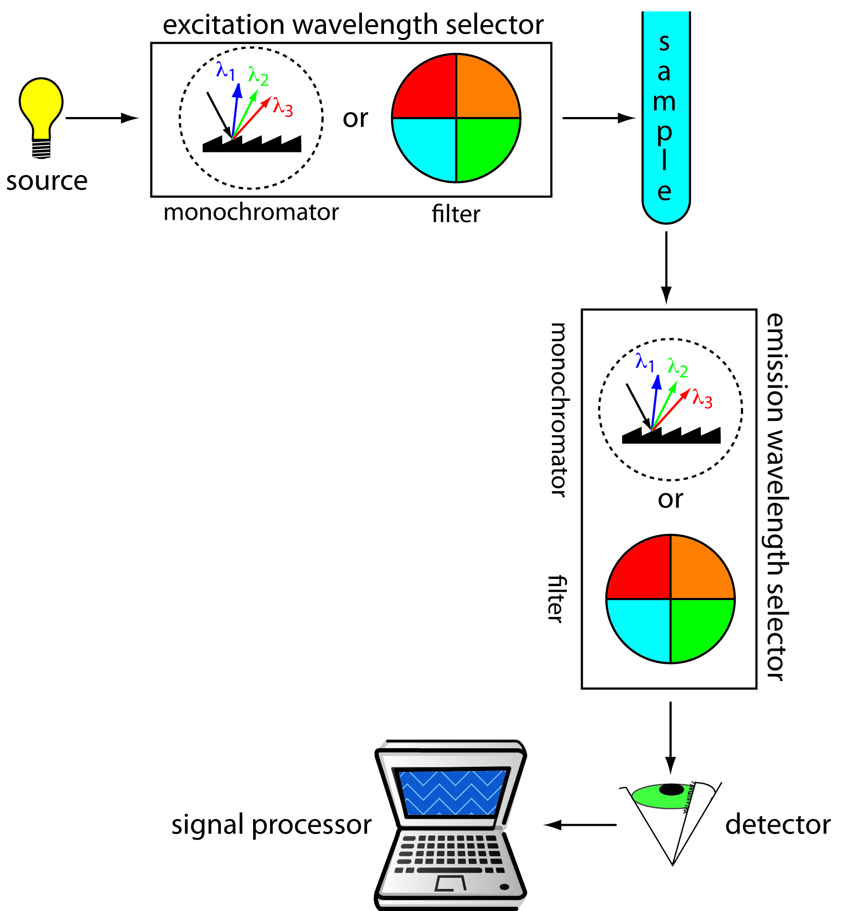
Figure 10.53 Schematic diagram for measuring fluorescence showing the placement of the wavelength selectors for excitation and emission. When a filter is used the instrument is called a fluorimeter, and when a monochromator is used the instrument is called a spectrofluorimeter.
The sample cells for molecular fluorescence are similar to those for molecular absorption. Remote sensing with fiber optic probes also can be adapted for use with either a fluorimeter or spectrofluorimeter. An analyte that is fluorescent can be monitored directly. For analytes that are not fluorescent, a suitable fluorescent probe molecule can be incorporated into the tip of the fiber optic probe. The analyte’s reaction with the probe molecule leads to an increase or decrease in fluorescence.
Instruments for Measuring Phosphorescence
Instrumentation for molecular phosphorescence must discriminate between phosphorescence and fluorescence. Because the lifetime for fluorescence is shorter than that for phosphorescence, discrimination is easily achieved by incorporating a delay between exciting the sample and measuring phosphorescent emission. Figure 10.54 shows how two out-of-phase choppers can be use to block emission from reaching the detector when the sample is being excited, and to prevent source radiation from reaching the sample while we are measuring the phosphorescent emission.

Figure 10.54 Schematic diagram showing how choppers are used to prevent fluorescent emission from interfering with the measurement of phosphorescent emission.
Because phosphorescence is such a slow process, we must prevent the excited state from relaxing by external conversion. Traditionally, this has been accomplished by dissolving the sample in a suitable organic solvent, usually a mixture of ethanol, isopentane, and diethylether. The resulting solution is frozen at liquid-N2 temperatures, forming an optically clear solid. The solid matrix minimizes external conversion due to collisions between the analyte and the solvent. External conversion also is minimized by immobilizing the sample on a solid substrate, making possible room temperature measurements. One approach is to place a drop of the solution containing the analyte on a small disc of filter paper. After drying the sample under a heat lamp, the sample is placed in the spectrofluorimeter for analysis. Other solid surfaces that have been used include silica gel, alumina, sodium acetate, and sucrose. This approach is particularly useful for the analysis of thin layer chromatography plates.
10.6.3 Quantitative Applications
Molecular fluorescence and, to a lesser extent, phosphorescence have been used for the direct or indirect quantitative analysis of analytes in a variety of matrices. A direct quantitative analysis is possible when the analyte’s fluorescent or phosphorescent quantum yield is favorable. When the analyte is not fluorescent or phosphorescent, or if the quantum yield is unfavorable, then an indirect analysis may be feasible. One approach is to react the analyte with a reagent to form a product with fluorescent or phosphorescent properties. Another approach is to measure a decrease in fluorescence or phosphorescence when the analyte is added to a solution containing a fluorescent or phosphorescent probe molecule. A decrease in emission is observed when the reaction between the analyte and the probe molecule enhances radiationless deactivation, or produces a nonemittng product. The application of fluorescence and phosphorescence to inorganic and organic analytes are considered in this section.
Inorganic Analytes
Except for a few metal ions, most notably UO2+, most inorganic ions are not sufficiently fluorescent for a direct analysis. Many metal ions may be determined indirectly by reacting with an organic ligand to form a fluorescent, or less commonly, a phosphorescent metal–ligand complex. One example is the reaction of Al3+ with the sodium salt of 2, 4, 3′-trihydroxyazobenzene-5′-sulfonic acid—also known as alizarin garnet R—which forms a fluorescent metal–ligand complex (Figure 10.55). The analysis is carried out using an excitation wavelength of 470 nm, monitoring fluorescence at 500 nm. Table 10.12 provides additional examples of chelating reagents that form fluorescent metal–ligand complexes with metal ions. A few inorganic nonmetals are determined by their ability to decrease, or quench, the fluorescence of another species. One example is the analysis for F– based on its ability to quench the fluorescence of the Al3+–alizarin garnet R complex.
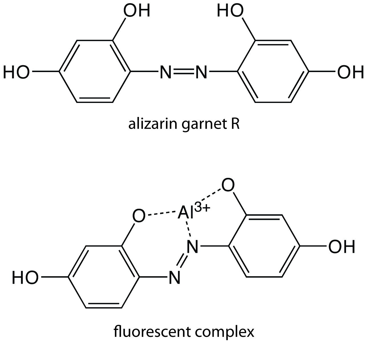
Figure 10.55 Structure of alizarin garnet R and its metal–ligand complex with Al3+.
| chelating agent | metal ions |
|---|---|
| 8-hydroxyquinoline | Al3+, Be2+, Zn2+, Li+, Mg2+ (and others) |
| flavonal | Zr2+, Sn4+ |
| benzoin | B4O72–, Zn2+ |
| 2', 3, 4′, 5, 7-pentahydroxyflavone | Be2+ |
| 2-(o-hydroxyphenyl) benzoxazole | Cd2+ |
Organic Analytes
As noted earlier, organic compounds containing aromatic rings generally are fluorescent and aromatic heterocycles are often phosphorescent. As shown in Table 10.13, several important biochemical, pharmaceutical, and environmental compounds may be analyzed quantitatively by fluorimetry or phosphorimetry. If an organic analyte is not naturally fluorescent or phosphorescent, it may be possible to incorporate it into a chemical reaction that produces a fluorescent or phosphorescent product. For example, the enzyme creatine phosphokinase can be determined by using it to catalyze the formation of creatine from phosphocreatine. Reacting the creatine with ninhydrin produces a fluorescent product of unknown structure.
| class | compounds (F = fluorescence; P = phosphorescence) |
|---|---|
| aromatic amino acids |
phenylalanine (F) |
| vitamins | vitamin A (F) vitamin B2 (F) vitamin B6 (F) vitamin B12 (F) vitamin E (F) folic acid (F) |
| catecholamines | dopamine (F) norepinephrine (F) |
| pharmaceuticals and drugs | quinine (F) salicylic acid (F, P) morphine (F) barbiturates (F) LSD (F) codeine (P) caffeine (P) sulfanilamide (P) |
| environmental pollutants | pyrene (F) benzo[a]pyrene (F) organothiophosphorous pesticides (F) carbamate insecticides (F) DDT (P) |
Standardizing the Method
From equation 10.28 and equation 10.29 we know that the intensity of fluorescent or phosphorescent emission is a linear function of the analyte’s concentration provided that the sample’s absorbance of source radiation (A = εbC) is less than approximately 0.01. Calibration curves often are linear over four to six orders of magnitude for fluorescence and over two to four orders of magnitude for phosphorescence. For higher concentrations of analyte the calibration curve becomes nonlinear because the assumptions leading to equation 10.28 and equation 10.29 no longer apply. Nonlinearity may be observed for small concentrations of analyte due to the presence of fluorescent or phosphorescent contaminants. As discussed earlier, quantum efficiency is sensitive to temperature and sample matrix, both of which must be controlled when using external standards. In addition, emission intensity depends on the molar absorptivity of the photoluminescent species, which is sensitive to the sample matrix.
Note
The best way to appreciate the theoretical and practical details discussed in this section is to carefully examine a typical analytical method. Although each method is unique, the following description of the determination of quinine in urine provides an instructive example of a typical procedure. The description here is based on Mule, S. J.; Hushin, P. L. Anal. Chem. 1971, 43, 708–711, and O’Reilly, J. E.; J. Chem. Educ. 1975, 52, 610–612.
Representative Method 10.3
Determination of Quinine in Urine
Description of Method
Quinine is an alkaloid used in treating malaria. It is a strongly fluorescent compound in dilute solutions of H2SO4 (Φf = 0.55). Quinine’s excitation spectrum has absorption bands at 250 nm and 350 nm and its emission spectrum has a single emission band at 450 nm. Quinine is rapidly excreted from the body in urine and is easily determined by measuring its fluorescence following its extraction from the urine sample.
(Figure 10.49 shows the fluorescence of the quinine in tonic water.)
Procedure
Transfer a 2.00-mL sample of urine to a 15-mL test tube and adjust its pH to between 9 and 10 using 3.7 M NaOH. Add 4 mL of a 3:1 (v/v) mixture of chloroform and isopropanol and shake the contents of the test tube for one minute. Allow the organic and the aqueous (urine) layers to separate and transfer the organic phase to a clean test tube. Add 2.00 mL of 0.05 M H2SO4 to the organic phase and shake the contents for one minute. Allow the organic and the aqueous layers to separate and transfer the aqueous phase to the sample cell. Measure the fluorescent emission at 450 nm using an excitation wavelength of 350 nm. Determine the concentration of quinine in the urine sample using a calibration curve prepared with a set of external standards in 0.05 M H2SO4, prepared from a 100.0 ppm solution of quinine in 0.05 M H2SO4. Use distilled water as a blank.
Questions
1. Chloride ion quenches the intensity of quinine’s fluorescent emission. For example, in the presence of 100 ppm NaCl (61 ppm Cl–) quinine’s emission intensity is only 83% of its emission intensity in the absence of chloride. The presence of 1000 ppm NaCl (610 ppm Cl–) further reduces quinine’s fluorescent emission to less than 30% of its emission intensity in the absence of chloride. The concentration of chloride in urine typically ranges from 4600–6700 ppm Cl–. Explain how this procedure prevents an interference from chloride.
The procedure uses two extractions. In the first of these extractions, quinine is separated from urine by extracting it into a mixture of chloroform and isopropanol, leaving the chloride behind in the original sample.
2. Samples of urine may contain small amounts of other fluorescent compounds, which interfere with the analysis if they are carried through the two extractions. Explain how you can modify the procedure to take this into account?
One approach is to prepare a blank using a sample of urine known to be free of quinine. Subtracting the blank’s fluorescent signal from the measured fluorescence from urine samples corrects for the interfering compounds.
3. The fluorescent emission for quinine at 450 nm can be induced using an excitation frequency of either 250 nm or 350 nm. The fluorescent quantum efficiency is the same for either excitation wavelength. Quinine’s absorption spectrum shows that ε250 is greater than ε350. Given that quinine has a stronger absorbance at 250 nm, explain why its fluorescent emission intensity is greater when using 350 nm as the excitation wavelength.
From equation 10.28 we know that If is a function of the following terms: k, Φf, P0, ε, b, and C. We know that Φf, b, and C are the same for both excitation wavelengths and that ε is larger for a wavelength of 250 nm; we can, therefore, ignore these terms. The greater emission intensity when using an excitation wavelength of 350 nm must be due to a larger value for P0 or k. In fact, P0 at 350 nm for a high-pressure Xe arc lamp is about 170% of that at 250 nm. In addition, the sensitivity of a typical photomultiplier detector (which contributes to the value of k) at 350 nm is about 140% of that at 250 nm.
Example 10.11
To evaluate the method described in Representative Method 10.3, a series of external standard was prepared and analyzed, providing the results shown in the following table. All fluorescent intensities were corrected using a blank prepared from a quinine-free sample of urine. The fluorescent intensities are normalized by setting If for the highest concentration standard to 100.
|
[quinine] (μg/mL) |
If |
|
1.00 |
10.11 |
|
3.00 |
30.20 |
|
5.00 |
49.84 |
|
7.00 |
69.89 |
|
10.00 |
100.0 |
After ingesting 10.0 mg of quinine, a volunteer provided a urine sample 24-h later. Analysis of the urine sample gives an relative emission intensity of 28.16. Report the concentration of quinine in the sample in mg/L and the percent recovery for the ingested quinine.
Solution
Linear regression of the relative emission intensity versus the concentration of quinine in the standards gives a calibration curve with the following equation.
\[I_\ce{f} = \mathrm{0.124 + 9.978 × \dfrac{g\: quinine}{mL}}\]
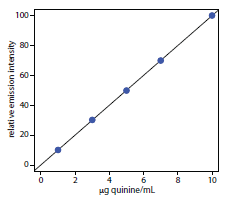
Substituting the sample’s relative emission intensity into the calibration equation gives the concentration of quinine as 2.81 μg/mL. Because the volume of urine taken, 2.00 mL, is the same as the volume of 0.05 M H2SO4 used in extracting quinine, the concentration of quinine in the urine also is 2.81 μg/mL. The recovery of the ingested quinine is
\[\mathrm{\dfrac{\dfrac{2.81\: g}{ml\: urine} × 2.00\: mL\: urine × \dfrac{1\: mg}{1000\: g}}{10.0\: mg\: quinine\: ingested} × 100 = 0.0562\%}\]
(It can take up 10–11 days for the body to completely excrete quinine.)
10.6.4 Evaluation of Photoluminescence Spectroscopy
Scale of Operation
Photoluminescence spectroscopy is used for the routine analysis of trace and ultratrace analytes in macro and meso samples. Detection limits for fluorescence spectroscopy are strongly influenced by the analyte’s quantum yield. For an analyte with Φf > 0.5, a picomolar detection limit is possible when using a high quality spectrofluorimeter. For example, the detection limit for quinine sulfate, for which Φf is 0.55, is generally between 1 part per billion and 1 part per trillion. Detection limits for phosphorescence are somewhat higher, with typical values in the nanomolar range for low-temperature phosphorimetry, and in the micromolar range for room-temperature phosphorimetry using a solid substrate.
Note
See Figure 3.5 to review the meaning of macro and meso for describing samples, and the meaning of major, minor, and ultratrace for describing analytes.
Accuracy
The accuracy of a fluorescence method is generally between 1–5% when spectral and chemical interferences are insignificant. Accuracy is limited by the same types of problems affecting other optical spectroscopic methods. In addition, accuracy is affected by interferences influencing the fluorescent quantum yield. The accuracy of phosphorescence is somewhat greater than that for fluorescence.
Precision
The relative standard deviation for fluorescence is usually between 0.5–2% when the analyte’s concentration is well above its detection limit. Precision is usually limited by the stability of the excitation source. The precision for phosphorescence is often limited by reproducibility in preparing samples for analysis, with relative standard deviations of 5–10% being common.
Sensitivity
From equation 10.28 and equation 10.29 we know that the sensitivity of a fluorescent or phosphorescent method is influenced by a number of parameters. The importance of quantum yield and the effect of temperature and solution composition on Φf and Φp already have been considered. Besides quantum yield, the sensitivity of an analysis can be improved by using an excitation source that has a greater emission intensity, P0, at the desired wavelength, and by selecting an excitation wavelength that has a greater absorbance. Another approach for improving sensitivity is to increase the volume in the sample from which emission is monitored. Figure 10.56 shows how rotating a monochromator’s slits from their usual vertical orientation to a horizontal orientation increases the sampling volume. The result can increase the emission from the sample by 5–30×.
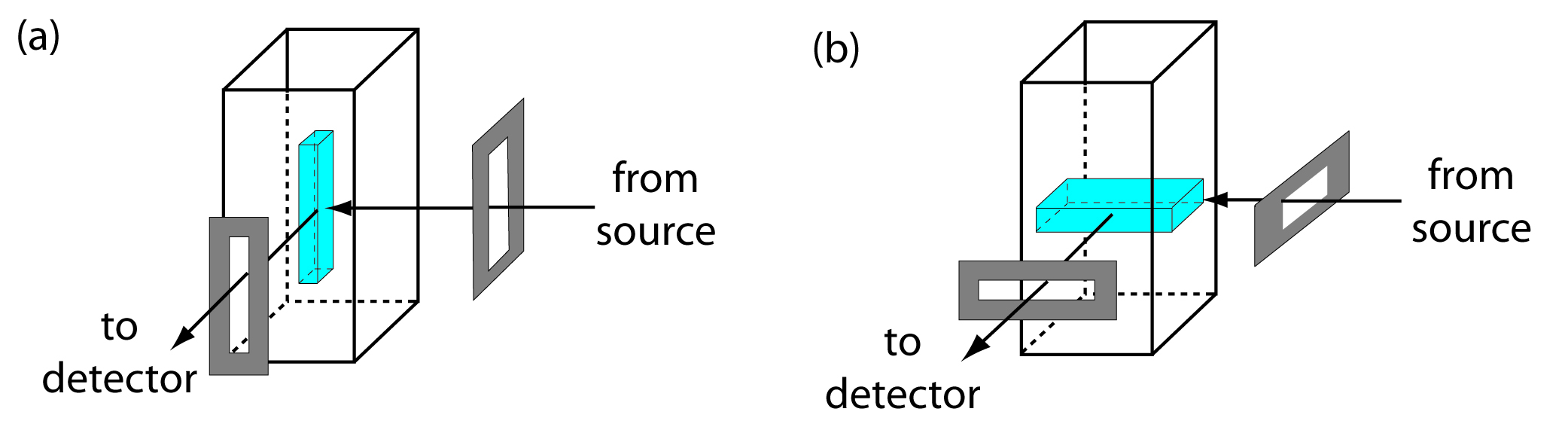
Figure 10.56 Use of slit orientation to change the volume from which fluorescence is measured: (a) vertical slit orientation; (b) horizontal slit orientation. Suppose the slit’s dimensions are 0.1 mm × 3 mm. In (a) the dimensions of the sampling volume are 0.1 mm × 0.1mm × 3 mm, or 0.03 mm3. For (b) the dimensions of the sampling volume are 0.1 mm × 3 mm × 3 mm, or 0.9 mm3, a 30-fold increase in the sampling volume.
Selectivity
The selectivity of fluorescence and phosphorescence is superior to that of absorption spectrophotometry for two reasons: first, not every compound that absorbs radiation is fluorescent or phosphorescent; and, second, selectivity between an analyte and an interferent is possible if there is a difference in either their excitation or their emission spectra. The total emission intensity is a linear sum of that from each fluorescent or phosphorescent species. The analysis of a sample containing n components, therefore, can be accomplished by measuring the total emission intensity at n wavelengths.
Time, Cost, and Equipment
As with other optical spectroscopic methods, fluorescent and phosphorescent methods provide a rapid means for analyzing samples and are capable of automation. Fluorimeters are relatively inexpensive, ranging from several hundred to several thousand dollars, and often are satisfactory for quantitative work. Spectrofluorimeters are more expensive, with models often exceeding $50,000.