Self-consistent field theory

An important unsolved problem in quantum mechanics is how to deal with indistinguishable, interacting particles - in particular electrons which determine the behavior of almost every object in nature. The basic problem is that if particles interact, that interaction must be in the Hamiltonian. So until we know where the particles are, we cannot write down the Hamiltonian, but until we know the Hamiltonian, we can’t tell where the particles are.

The idea is to solve the Schrödinger equation for an electron moving in the potential of the nucleus and all the other electrons. We start with a guess for the trial electron charge density, solve Z/2 one-particle Schrödinger equations (initially identical) to obtain Z electron wavefunctions. Then we construct the potential for each wavefunction from that of the nucleus and that of all the other electrons, symmetrize it, and solve the Z/2 Schrödinger equations again. Fock improved on Hartree’s method by using the properly antisymmetrized wavefunction (Slater determinant) instead of simple one-electron wavefunctions. Without this, the exchange interaction is missing. This method is ideal for a computer, because it is easily written as an algorithm.

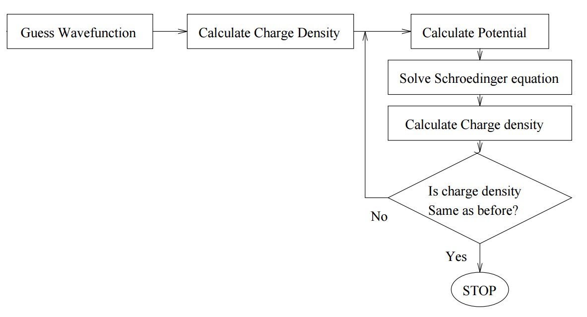
Figure \(\PageIndex{1}\): Algorithm for Self-consistent field theory.

Although we are concerned here with atoms, the same methodology is used for molecules or even solids (with appropriate potential symmetries and boundary conditions). This is a variational method, so wherever we refer to wavefunctions, we assume that they are expanded in some appropriate basis set. The full set of equations are

The first term is the kinetic energy and electron-ion potential. The second “Hartree” term, is the electrostatic potential from the charge distribution of N electrons, including an unphysical self-interaction of electrons when \(j = i\). The third, “exchange” term, acts only on electrons with the same spin and comes from the Slater determinant form of the wavefunction. Physically, the effect of exchange is for like-spin electrons to avoid each other. Each electron is surrounded by an “exchange hole”: there is one fewer like-spin electrons nearby than the mean-field would imply. The term \(i = j\) neatly cancels out the self interaction of the electron.

Electron Correlation and the "Exchange Hole"

Hartree-Fock theory does not properly describe correlation. In the Copenhagen Interpretation, the squared modulus of the wavefunction gives the probability of finding a particle in a given place. The many-body wave function gives the N-particle distribution function, i.e. \(|Φ(r_1, ..., r_N )|^2\) is the probability density that particle 1 is at \(r_1\), ..., and particle \(N\) is at \(r_N\). But when trying to work out the interaction between electrons, what we want to know is the probability of finding an electron at \(r\), given the positions of all the other electrons \(\{r_i\}\). This implies that the electron behaves quantum mechanically when we evaluate its wavefunction, but as a classical point particle when it contributes to the potential seen by the other electrons.

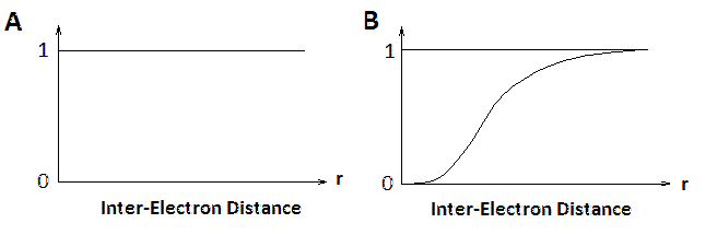
Figure \(\PageIndex{2}\): Normalized Conditional Probability of n(r) for from electron-electron interactions (excluding coulomb effects) in (A) the Hartree approximation and (B) the Hartree-Fock approximation.

The contributions of electron-electron interactions in N-electron systems within the Hartree and Hartree-Fock methods are shown in Figure \(\PageIndex{2}\). The conditional electron probability distributions \(n(r)\) of \(N-1\) electrons around an electron with given spin situated at \(r=0\). Within the Hartree approximation, all electrons are treated as independent, therefore \(n(r)\) is structureless. However, within the Hartree-Fock approximation, the \(N\)-electron wavefunction reflects the Pauli exclusion principle and near the electron at \(r=0\) the exchange hole can be seen where the the density of spins equal to that of the central electron is reduced. Electrons with opposite spins are unaffected (not shown).

Contributors

• Template:ContribAukland