1.1: Stability of Conjugated Dienes- Molecular Orbital Theory

Objectives

After completing this section, you should be able to

1. Write a reaction sequence to show a convenient method for preparing a given conjugated diene from an alkene, allyl halide, alkyl dihalide or alcohol (diol).
2. Identify the reagents needed to prepare a given diene from one of the starting materials listed in Objective 1, above.
3. Compare the stabilities of conjugated and non-conjugated dienes, using evidence obtained from hydrogenation experiments.
4. Discuss the bonding in a conjugated diene, such as 1,3-butadiene, in terms of the hybridization of the carbon atoms involved.
5. Discuss the bonding in 1,3-butadiene in terms of the molecular orbital theory, and draw a molecular orbital for this and similar compounds.

Synthesis of Dienes

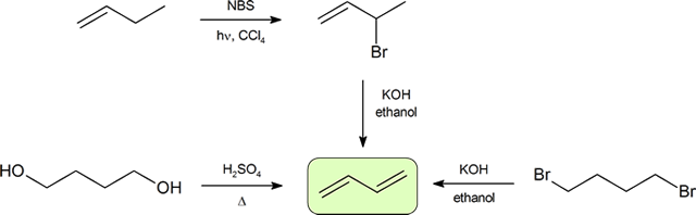
Conjugated dienes can be prepared using many of the methods used for the preparation of alkenes previously discussed (Organic Chemistry I Section 8.3). A convenient method starts with the free radical halogenation of the allylic carbon of an alkene using NBS. The resulting halide can then be reacted with a strong base to result in E2 elimination and create a diene product. The compound, 1,3-butadiene, is the simplest conjugated diene and has an important use in the synthesis of polymers which will be discussed in Section 1.7. Many simple dienes, such as 1,3-butadiene and isoprene, can be prepared industrially by the double dehydration of alcohols and the double dehydrohalogenation of organohalides.

 

Stability of Conjugated Dienes

Conjugated dienes are known to be more stable than non-conjugated dienes, as shown by their experimentally determined heats of hydrogenation. In Organic Chemistry I Section 7-6, it was shown that as alkenes become more stable, they contain less energy, and therefore release less heat during hydrogenation.

Table \(\PageIndex{1}\): Heats of Hydrogenation for Some Alkenes and Dienes

Alkene or diene	Product	\(\Delta H^{\circ}_{\text{hydrog}}\)		Classification
		(kJ/mol)	(kcal/mol)
		–126	–30.1	Terminal Alkene
		–119	–28.4	More substituted Terminal Alkene
		–253	–60.5	Isolated diene
		–236	–56.4	Conjugated diene
		–229	–54.7	More substituted   Conjugated diene

Because a monosubstituted alkene has a \(\Delta H^{\circ}_{\text{hydrog}}\) of approximately –126 kJ/mol, (Table \(\PageIndex{1}\)), we might expect that a compound with two monosubstituted double bonds would have a \(\Delta H^{\circ}_{\text{hydrog}}\) approximately twice that value, or –252 kJ/mol. Non-conjugated dienes, such as 1,4-pentadiene (\(\Delta H^{\circ}_{\text{hydrog}}\) =−253 kJ/mol), meet this expectation, but the conjugated diene 1,3-butadiene (\(\Delta H^{\circ}_{\text{hydrog}}\)=−236 kJ/mol) does not. 1,3-Butadiene is approximately 16 kJ/mol (3.8 kcal/mol), more stable than expected.

Combination of Stabilization Factors

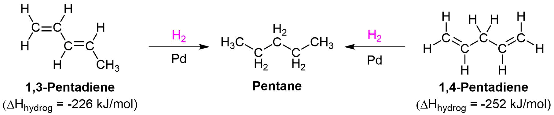
Experiments have shown that conjugated dienes have a lower heat of hydrogenation (-226 kJ/mol) than non-conjugated dienes (-253 kJ/mol). Using the differences in heat of hydrogenation, the stabilization energy for 1,3-pentadiene is approximately 27 kJ/mol, which accounts not only for the conjugation of the diene, but the additional substituent of the second double bond.

Here is an energy diagram comparing different types of bonds with their heats of hydrogenation to show the relative stability of each molecule:

Resonance forms of Conjugated Dienes

What accounts for the stability of conjugated dienes? According to valence bond theory (Organic Chemistry I, Section 1.5 and Section 1.8), their stability is due to orbital hybridization. Each alkene carbon are sp² hybridized and therefore have one unhybridized p orbital. In 1,3 dienes, like 1,3-butadiene, the four p orbitals  overlap to form a conjugated system which can be represented by the resonance forms shown below. This delocalization of charges stabilizes conjugated diene, making them more stable than non-conjugated dienes.

 

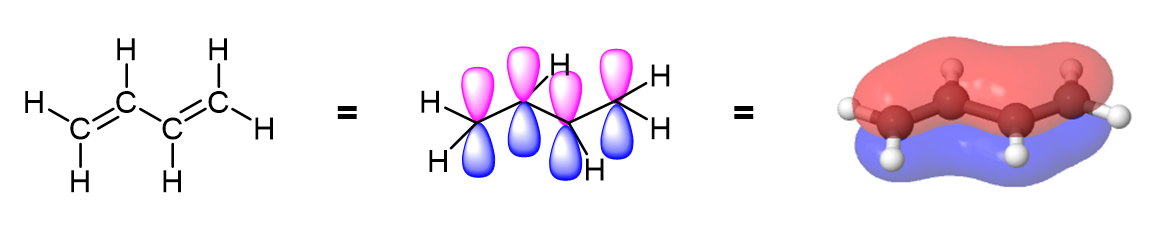
The delocalized electron density of a 1,3 diene can be seen in the electrostatic potential maps. In conjugated dienes, it is observed that the pi electron density overlap (shown in red) is closer together and delocalized in conjugated dienes, while in non-conjugated dienes the pi electron density is located completely on the double bonds.

Molecular Orbitals of 1,3 Dienes

According to MO theory, when a double bond is non-conjugated, the two atomic 2p_z orbitals combine to form two pi (π) molecular orbitals, one a low-energy π bonding orbital and one a high-energy π-star (π*) anti-bonding molecular orbital. These are sometimes denoted, in MO diagrams like the one below, with the Greek letter psi (Ψ) instead of π. In the bonding Ψ₁ orbital, the two (+) lobes of the 2p_z orbitals interact constructively with each other, as do the two (-) lobes. Therefore, there is increased electron density between the nuclei in the molecular orbital – this is why it is a bonding orbital. In the higher-energy anti-bonding Ψ₂* orbital, the (+) lobes of one 2p_z orbital interacts destructively with the (-) lobe of the second 2p_z orbital, leading to a node between the two nuclei and overall repulsion. By the aufbau principle, the two electrons from the two atomic orbitals will be paired in the lower-energy Ψ₁orbital when the molecule is in the ground state.

Figure \(\PageIndex{1}\): Two p orbitals combine to form two \(\pi\) molecular orbitals. Both electrons occupy the low-energy, bonding orbital, leading to a net lowering of energy and formation of a stable bond. The asterisk on \(ψ_2^{*}\) indicates an antibonding orbital.

Now let’s combine four adjacent p atomic orbitals, as occurs in a conjugated diene. With a conjugated diene, such as 1,3-butadiene, the four 2p atomic orbitals combine to form four pi molecular orbitals of increasing energy. Two bonding pi orbitals and two anti-bonding pi* orbitals. The combination of four pi molecular orbitals allow for the formation of a bonding molecular orbital that is lower in energy than those created by an unconjugated alkene. The 4 pi electrons of 1,3-butadiene completely fill the bonding molecular orbitals giving is the additional stability associated with conjugated double bonds.

Figure \(\PageIndex{2}\): Four \(\pi\) molecular orbitals in 1,3-butadiene. Note that the number of nodes between nuclei increases as the energy level of the orbital increases (from 0 to 3 nodes).

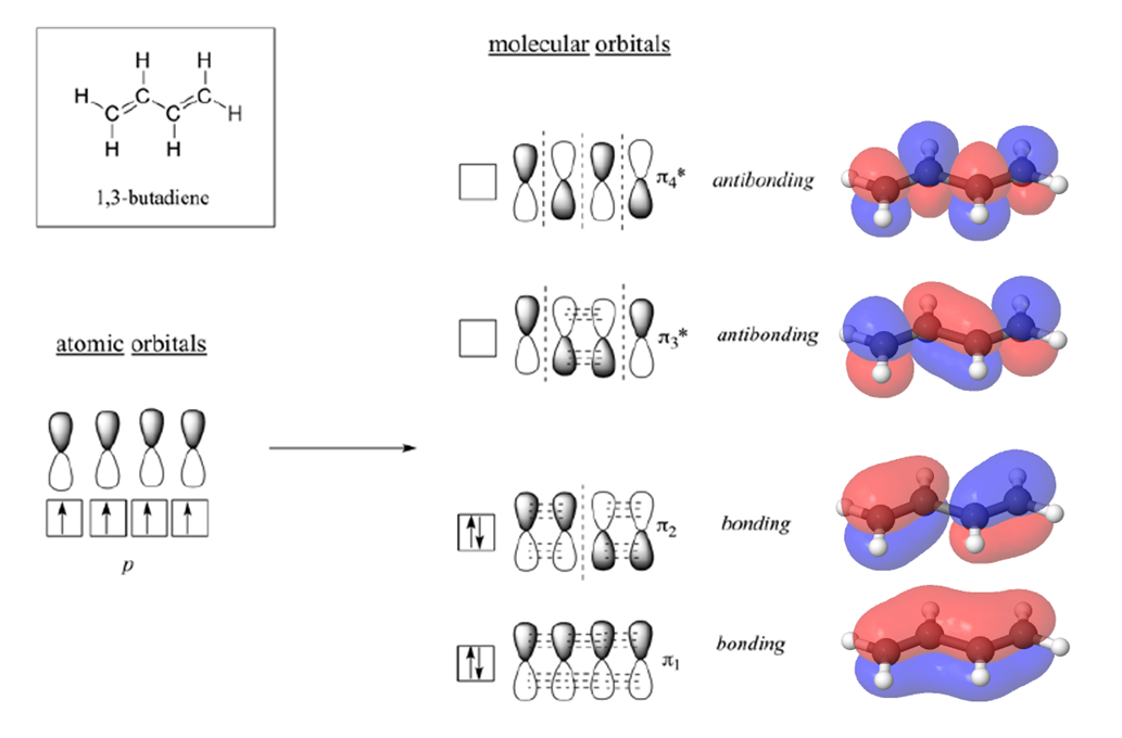
The lowest-energy \(\pi\) molecular orbital (denoted \(ψ_1\), Greek psi) has no nodes between the nuclei and is therefore bonding. The \(\pi\) MO of next-lowest energy, ψ2, has one node between nuclei and is also bonding. Above \(ψ_1\) and \(ψ_2\) in energy are the two antibonding \(\pi\) MOs, \(ψ_3^{*}\) and \(ψ_4^{*}\). (The asterisks indicate antibonding orbitals.) Note that the number of nodes between nuclei increases as the energy level of the orbital increases. The \(ψ_3^{*}\) orbital has two nodes between nuclei, and \(ψ_4^{*}\), the highest-energy MO, has three nodes between nuclei.

In describing 1,3-butadiene, we say that the \(\pi\) electrons are spread out, or delocalized, over the entire \(\pi\) framework, rather than localized between two specific nuclei. Delocalization allows the bonding electrons to be closer to more nuclei, thus leading to lower energy and greater stability.

Exercise \(\PageIndex{1}\)

Allene, H₂C=C=CH₂, has a heat of hydrogenation of –298 kJ/mol (–71.3 kcal/mol). Rank a conjugated diene, a nonconjugated diene, and an allene in order of stability.

Answer

Expected \(\Delta H^{\circ}_{\text{hydrog}}\) for allene is −252 kJ/mol. Allene is less stable than a nonconjugated diene, which is less stable than a conjugated diene.

Key Terms

Make certain that you can define, and use in context, the key terms below.

• delocalized electrons
• node

Study Notes

The two most frequent ways to synthesize conjugated dienes are dehydration of alcohols and dehydrohalogenation of organohalides, which were introduced in the preparation of alkenes (Organic Chemistry I Section 8.3). The following scheme illustrates some of the routes to preparing a conjugated diene.

The formation of synthetic polymers from dienes such as 1,3-butadiene and isoprene is discussed in Section 14.6. Synthetic polymers are large molecules made up of smaller repeating units. You are probably somewhat familiar with a number of these polymers; for example, polyethylene, polypropylene, polystyrene and poly(vinyl chloride).

As the hydrogenation of 1,3-butadiene releases less than the predicted amount of energy, the energy content of 1,3-butadiene must be lower than we might have expected. In other words, 1,3-butadiene is more stable than its formula suggests.

Figure \(\PageIndex{3}\):Energy diagram for the hydrogenation of 1,3-butadiene (not to scale).