5.5: Effects of the Sample, Equipment and Recording Regimes on the NMR Spectral Sensitivity and Resolution.

This Chapter describes how key elements of NMR data collection (properties of sample molecules, their concentration, magnet strength \(B_o\), recording regimes) affect the two fundamental qualities of the recorded data: spectral resolution and spectral sensitivity.

Learning Objectives

• Appreciate the effect of the magnetic field strength \(B_o\) on FID S₀ and spectral line intensity
• Develop a sense of difference between the signal and noise parts of NMR spectra
• Understand the link between the number of times the spectrum is recorded and spectral sensitivity
• Explore the connection between the magnetic field strength \(B_o\) and spectral resolution: linewidth in ppm and Hz vs peak separation in ppm and Hz
• Grasp the effects of the biomolecule size and concentration on the spectral line width and intensity

In the last practice problem of the previous Chapter, we applied Fourier transformation to a model FID originating from a single spin-½ system (nucleus). The resulting mathematical expression describing the NMR signal line-shape as a function of resonance angular frequency ω (=2⋅π⋅ν, where ν is the linear resonance frequency) is as follows:

Equation V.5.\ref{EQ:ls1}

\[\begin{eqnarray}I(\omega) &=& S _0 \frac{R}{R^2 + (\omega – \Omega)^2}\label{EQ:ls1}\end{eqnarray}\]

In this expression, the three parameters S₀, R, and Ω have exactly the same meaning as in Equation V.3.2 for FID (Chapter V.3) : initial current, FID relaxation rate and resonance frequency respectively. Equation V.5.1 above allows us to appreciate the effects of the sample properties, concentration and magnet power \(B_o\) on the key properties of the respective NMR resonance line: its position, intensity and line-width.

Magnet Strength B₀ and Signal Intensity

The intensity of the current detected in response to an NMR excitation by a particular sample (spin-½ system) is defined by the fraction of spins, S_up, whose spin projection on the axis of \(B_o\) is parallel to the field and which have no compensatory "anti-parallel" spins under the initial condition of thermal equilibrium (for positive gyromagnetic ratio values):

Equation V.5.\ref{EQ:pr2}

\[\begin{eqnarray}S _{up} &=& \frac {N(+1/2) – N(-1/2)}{N(+1/2) + N(-1/2)}\label{EQ:pr2}\end{eqnarray}\]

Utilizing the Boltzmann distribution formula for the ratio of spin-up over spin-down populations (Equation 5.1.3 in Chapter V.1), it can be shown that

Equation V.5.\ref{EQ:pp3}

\[\begin{eqnarray}S _{up} &=& \frac {1}{2} \cdot \frac { \Delta E }{ k \cdot T } \\[4pt] S _{up} &=& \frac {1}{2} \cdot \frac { h \cdot \gamma \cdot B _0 }{ k \cdot T }\label{EQ:pp3}\end{eqnarray}\]

Thus, we can see that the excess of the spin-up over spin-down populations is directly proportional to the value of gyromagnetic ratio γ and magnetic filed strength \(B_o\). (NB! this is a serious oversimplification) The initial signal intensity S₀ and thus NMR peak intensity can be viewed as directly proportional to S_up ratio. Under these assumptions, we can state that doubling the magnetic field \(B_o\) leads to doubling the signal intensity.

Signal-to-Noise Ratio as a Measure of Spectral Sensitivity

The Free Induction Decay (FID) recorded as electric current in every NMR experiment consists of two major components: the currents induced by alternating magnetic moment of the sample (that is “signal” itself) and random, stochastic electric currents existing in every electronic circuit also known as “noise”. The level of noise is defined by the properties of conductor and semiconductor elements of the circuits and temperature at which the electronics operates: the higher the temperature, the stronger the random noise currents. Unlike the noise, the signal from the sample is repeatable and if we rerun the NMR experiment, we will get exactly the same currents from the sample FID.

Spectral sensitivity is a measure of spectrum quality in the sense of the capacity of the scientist to distinguish the real peaks (signals) from noise. Figure V.5.A demonstrates how two spectra having very similar level (intensity) of its signals can differ in their capacity to distinguish real signals from elements of noise (see the features marked by red arrows).

Figure V.5.A The two spectra are similar in many respects except for their clarity about the features marked by the arrows. Peak on the left leaves plenty of doubts whether this feature is a real peak or it is a noise component. The spectrum on the right has generally a lower level of noise with respect to the signals and is unambiguous regarding the nature of the feature marked by the arrow: it is a real peak. The recordings were made by S.L. Smirnov.

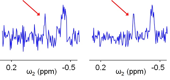
Figure V.5.A helps to appreciate why signal-to-noise (S/N) ratio is commonly used as a quantitative measure of spectral sensitivity. The higher the S/N ratio, the less the features of the noise can mask “real” peaks. Alternatively, the greater the S/N ratio, the smaller “real” signals can be identified.

Key Result: The S/N ratio offers a very practical approach to increase the sensitivity of NMR spectra: repeat recordings multiple (n) times and sum up the obtained spectra (the spectra can be summed up since Fourier transformation is a linear mathematical operation). Such a treatment will help to increase S/N ratio because the intensity of the real signals will be increased by factor n (“real” peaks will reproduce faithfully with every repetition of the experiment) , whereas the noise features being random or stochastic will have their intensities increased on average by a factor n^0.5 (square root or n). Thus after the recording is repeated n times, signal-to-noise ratio will grow as n/n^0.5 = n^0.5. For example, to increase spectra sensitivity by factor 2, one needs to repeat the recording 4 times (2 = 4^0.5).

Repeating NMR recordings multiple times offers a way to increase spectral sensitivity while working with the same instrumentation (that is without resorting to more powerful and thus less accessible spectrometers). Another obvious way to increase spectra sensitivity is to use a more powerful magnet (with greater \(B_o\) ) as Equation V.5.3 above suggests. This way, the signal intensity will go up proportionately to B0 or even faster. If the noise level stays the same, S/N will be greater. The same Equation V.5.3 offers another avenue: alter the temperature (up? down?) to get stronger signal and greater S/N ratio. Increasing the amount of the sample used for the recording is another general and widely used way to increase the intensity of the signals while keeping the noise level the same (the noise level depends on the instrumentation and not on the amount of the sample in the NMR tube).

Broader picture: In addition to the generally used ways to increase sensitivity of NMR spectra listed above, more sensitive NMR probes have appeared as the most recent method to increase S/N of NMR recordings. Such probes are often referred to as cryoprobes since their electronics is cooled by liquid cryogens (e.g. helium or nitrogen) to drive the circuitry temperature and noise currents down. The temperature of the sample in an NMR cryoprobe is still controlled by the operator: in other words, in cryoprobes our biomolecular samples are not cryogen-cold.

Sample Relaxation Rates: Effects on Spectral Sensitivity and Resolution

Sensitivity: Equation V.5.1 above shows that the NMR peak intensity depends on the value of the FID relaxation rate R. This means that if for whatever reason the overall relaxation rate of a particular spin-½ changes, the signal intensity and this spectral sensitivity will change. There are multiple reasons, which can lead to alteration in rates of FID relaxation (to be discussed later in this text). Some of those reasons include: larger or smaller size of the biological molecule, a polypeptide adopting more folded or more disordered conformation, certain conformational or chemical exchanges phenomena etc. Algebraically, I(\(\omega\) ) goes down as the relaxation rate R goes up. This spectral sensitivity goeas up when the FID relaxes slower and goes down when the relaxation rates increase. Example 1 below provides a quick introduction into this relationship.

Resolution: Spectral resolution described the capacity of the operator tell two adjacent peaks apart. In other words, the user of the spectrum needs to know whether a particular spectral pattern shows a single peak or two peaks or three or more. Likewise, it is important to be able to determine the peak position (Ω values) and spectra of sufficient resolution allow this.

Examples

Example 1. What is the effect of doubling the relaxation rate R on spectral sensitivity?

Sensitivity can be quantified as the S/N ratio. Since we are discussing in this example changes in the properties of the sample, the noise level (property of the instrument) remains constant. According to Equation V.5.1 above, the peak intensity at \(\omega\) = Ω, I(\(\omega\) ) = S₀/R. This increasing the relaxation rates by factor 2 (e.g. if the sample dimerize) will lead to reduction in signal intensities by factor 2. Thus with the noise level staying constant, S/N ratio and sensitivity will drop by factor 2.

Example 2. What is the effect of doubling the relaxation rate R on spectral resolution? Consider the case of two NMR signals of the same S₀ value and separated by 100 Hz. For both of them, let their relaxation rates be 20 Hz initially and twice that value after a certain change (the separation between the peak position and S₀ values remain the same).

Will the two peaks be better resolved or worse resolved after their respective relaxation rates double?

Equation V.5.1 above shows the at greater R (while S₀ and the Ω stay the same), the peak will be generally broader: do Practice Problem 4 as a hint to appreciate the effect of R. Thus as the R values double, the peaks’ shoulders get closer to and peaks become less resolved.

Practice Problems

Problem 1. Calculate the S_up value for ¹H spins for NMR recordings performed at 25 ^oC and magnetic field value a) \(B_o\) = 11.7 tesla and b) \(B_o\) = 23.4 Tesla

Problem 2. Build in Excel a graph showing an NMR spectral lineshape as a function of angular frequency ω for spin-½ system with the following parameters: S₀ = 1, Ω = 1000 rad/sec, R = 10 Hz

Problem 3. Predict how the changes in the line-shape in Problem 2 if the amount of the sample is doubled. Specifically, how will the following properties change ? a) peak position? b) peak height ? c) peak width?

Problem 4*. Spectral resolution is greater for spectra with narrower (sharper) peaks. NMR peak width is often reported as linewidth at half-height (LWHH). Utilize Equation V.5.1 above to determine how each of the three key parameters describing an NMR peak (S₀, R and Ω) affect LWHH of a peak?

Problem 5. The NMR frequency axis can be labeled in ppm or Hz (the two most common types of units). Consider a sample with just two NMR resonances (peaks). If two NMR recordings are done at B₀ values of 300 MHz and 600 MHz (¹H frequency), what is the change in peak separation and LWHH values at the two field strength if expressed in units of ppm? Same question if the x-axis units are Hz?