2.3: Transition State Theory

Thus far we have not considered the temperature dependence of the rate. Temperature affects a reaction rate because the rate “constant” \(k\) that enters into the rate equation is temperature dependent. Typically, the rate of a reaction will increase with temperature because a higher kinetic energy leads to more molecular collisions with sufficient orientation and energy. However, for enzyme-catalyzed reactions, a higher temperature can lead to a decrease in the rate as the enzyme denatures at higher temperatures. In this chapter we discuss how the rate of a reaction depends on the temperature and on the activation energy. This will lead to a discussion on transition state theory. In transition state theory a reaction proceeds through a high-energy intermediate whose formation is a kinetic bottleneck, making the reaction a rare event.

Learning Objectives

• Understand how the rate constant depends on temperature and be able to calculate the change in the rate at two different temperatures, given the activation energy.
• Understand the meaning of the potential energy surface and how it can be used as a reaction coordinate for simple reactions.
• Be able to use transition state theory to provide a meaning to the terms in the Arrhenius equation and to relate the rate constant to thermodynamic properties.

Temperature dependence of Rate

For a typical reaction, A + B → products, (shown in Figure II.3.A), the reaction requires the reactants A and B to collide with sufficient energy at the correct orientation in space. The rate law for this second order reaction is:

\[\text{rate} = k \left[ A \right] \left[B \right]\label{EQ:rate1}\]

One can image that as the temperature increase the kinetic energy of the molecules increases and so does the number of collisions with sufficient energy. Thus, the rate typically increases as the temperature is increased. The Arrhenius equation describes the usual observed dependence of the rate constant \(k\) with the temperature:

\[k = A e^{-E_a/RT}\label{EQ:Arrhenius}\]

where \(T\) is the temperature, \(E_a\) is the activation energy, \(R\) is the gas constant (in J mol\(^{-1}\) K\(^{-1}\)), and \(A\) is a pre-exponential factor. Taking the natural log of both sides of Equation \ref{EQ:Arrhenius} gives a linearized form:

\[\ln k = \ln A – \frac{E_a}{RT}\label{EQ:linear1}\]

A plot is shown in Figure II.3.A, where the slope gives the activation energy \(E_a/R\) and the intercept is the \(\ln A\).

Figure II.3.A. Plot of \(\ln k\) vs. 1/T. For Arrhenius behavior, the plot is linear with a slope equal to \(-E_a/R\).

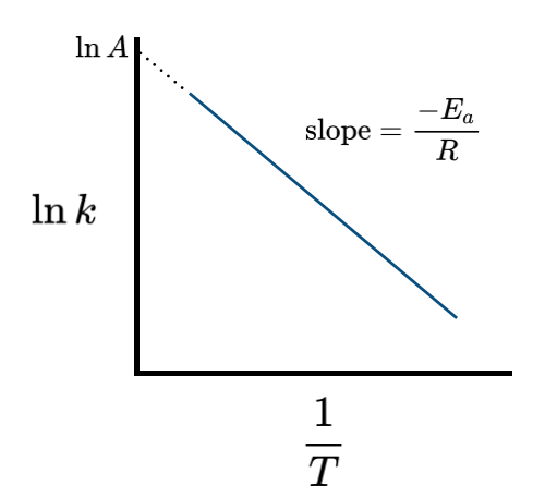
If the rate constant \(k\) can be measured at two temperatures, \(T_1\) and \(T_2\), then the pre-exponential factor drops out of Equation \ref{EQ:linear1}, giving:

\[\ln \frac{k_2}{k_1} = – \frac{E_a}{R}\left(\frac{1}{T_2}-\frac{1}{T_1}\right)\label{EQ:linear2}\]

See practice problem 1

Potential energy surface

To better understand the concept of the activation energy, we turn to a discussion of the potential energy surface and the energetics of a reaction. A simple reaction diagram is shown in Figure II.3.B which shows the energy of the reactants, transition state, and products along a hypothetical reaction coordinate. The reaction coordinate is a representation of the degree to which a reaction has progressed.

Figure II.3.B. The potential energy for the H₂ molecule as a function of the internuclear distance r. The minimum in energy corresponds to the equilibrium bond length.

A simple way to think about the reaction coordinate is to consider the combination of two atoms to form a diatomic molecule, such as H + H → H₂. The potential energy curve describing the interaction energy between the H atoms is shown in Figure II.3.B. At large distances, the individual atoms do not feel each other. As the distance between them decreases, there is a net attraction leading to a stable bond formation in the H₂ molecule. For a slightly more complex reaction, such as the substitution of a halogen via the SN₂ mechanism:

\[\ce{Cl^{–} + Br-CH3 → Br^{–} + Cl-CH3}\nonumber\]

a three-dimensional potential energy surface plot is required. Figure II.3.C shows a hypothetical potential energy surface for this reaction.

Figure II.3.C. A contour plot of the two dimensional potential energy surface for the SN₂ reaction Cl^– + Br-CH₃ → Br^– + Cl-CH₃. The red line traces the path along the minimum energy between reactant and product. The reaction proceeds via an activated complex located at the red dot between the reactant and product.

The potential energy curve for the formation of the Cl-CH₃ bond is plotted along the y-axis, and the potential energy curve for the formation of the Br-CH₃ bond is plotted along the x-axis. The contour plot shows the energies corresponding to different combinations of the atomic distances \(R_{C-Br}\) and \(R_{C-Cl}\). The red curve traces out the minimum amount of energy along a reaction path from reactants to products. The minimum energy path has a saddle point that represents the location of the activated complex [Cl ··· CH₃ ··· Br]. The minimum potential energy path can be represented as the reaction coordinate shown in Figure II.3.D.

Figure II.3.D. A one dimensional reaction coordinate along the minimum in energy path given by the red curve in Figure II.3.C. The formation of the high-energy activated complex at the energy barrier is the rate limiting step.

Transition state theory

In Equation \ref{EQ:Arrhenius} we introduced two parameters: the pre-exponential factor \(A\) and the activation energy \(E_a\). These value of these parameters determine the temperature dependence of the rate constant. In this section, we will consider one theory of reaction dynamics (transition state theory) to account for these parameters in the Arrhenius equation. Transition state theory can be used to explain the rates of biochemical reactions in fluid environments and provides insight into the details of a reaction at the molecular scale.

Transition state theory assumes that as two reactants come together, the potential energy increases and reaches a maximum. The maximum corresponds to the formation of an activated complex that can either continue on to form the products or can collapse back to the reactants. Consider a reaction of the form of Reaction Scheme 1:

\[\ce{A + B <=> [AB^{\ddagger}] -> P} \nonumber\]

where \(\ce{A}\) and \(\ce{B}\) are reactants that form an activated complex \(\ce{[AB^{\ddagger}]}\) that can collapse back into \(\ce{A}\) and \(\ce{B}\) or continue to products, \(\ce{P}\). If the reactants \(\ce{A + B}\) are at equilibrium with the activated complex, an equilibrium constant can be defined as

\[K^{\ddagger} = \frac{[AB^{\ddagger}]}{[A][B]}\label{EQ:ts1}\]

The rate of the reaction is proportional to the concentration of the activated complex [AB\(^{\ddagger}\)] at the top of the energy barrier. It follows that the rate constant can be written as:

\[k = \kappa \nu K^{\ddagger}\label{EQ:Eyring1}\]

where \(\nu\) is the frequency of vibration of the activated complex along the degree of freedom that leads to the formation of the product. (From statistical thermodynamics it can be shown that the vibrational frequency is \(\nu = k_BT/h\) where \(k_B\) is Boltzmann’s constant and \(h\) is Planck’s constant). The parameter \(\kappa\) is called the transmission coefficient and is introduced to account for the fact that the activated complex does not always form product.

The rate constant in Equation \ref{EQ:Eyring1} can be related to the thermodynamic properties through the relation:

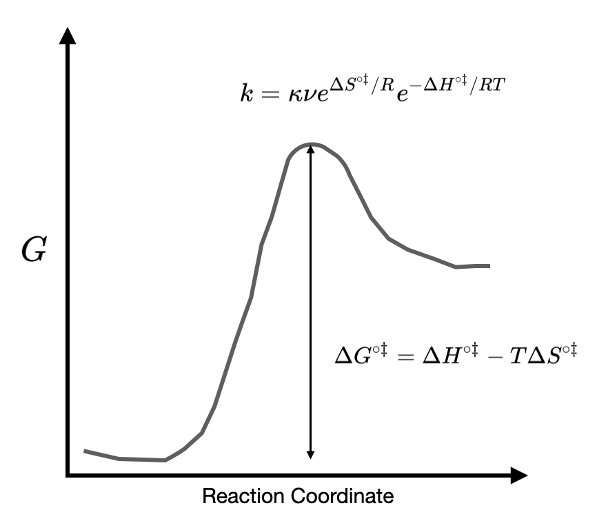
\[\Delta G^{\circ \ddagger} = -RT \ln K^{\ddagger}\label{EQ:thermoDeltaG}\]

where \(\Delta G^{\circ \ddagger}\) is the change in standard molar Gibbs energy of activation as shown in Figure X. Combining Equation \ref{EQ:thermoDeltaG} and Equation \ref{EQ:Eyring1} gives an expression for the rate constant:

\[\begin{align} k&= \kappa \nu e^{-\Delta G^{\circ \ddagger}/RT} \nonumber \\[4pt] &= \kappa \nu e^{\Delta S^{\circ \ddagger}/R}e^{-\Delta H^{\circ \ddagger}/RT}\label{EQ:TStheory}\end{align}\]

where in the second line we have used the fact that \(\Delta G^{\circ \ddagger} = \Delta H^{\circ \ddagger}-T\Delta S^{\circ \ddagger}\). Comparing Equation \ref{EQ:TStheory} with the Arrhenius equation Equation \ref{EQ:Arrhenius} we see that the pre-exponential factor \(\bf{A}\) is given by transition state theory to be

\[A=\kappa \nu e^{\Delta S^{\circ \ddagger}/R}\label{EQ:A}\]

and the activation energy \(\bf{E_a}\) is identified as the enthalpy of activation \(\Delta H^{\circ \ddagger}\) as shown in Figure II.3.E.

Figure II.3.E. Gibbs energy change for a reaction. The standard molar Gibbs energy of activation \(\Delta G^{\circ \ddagger}\) is the difference in Gibbs energy between the activated complex and the reactant.

Practice Problems

Problem 1. What is the rate constant at 300 K for a reaction with activation energy \(E_a = 50\) J mol\(^{-1}\) and a pre-exponential factor of \(A=10^{11}\) s\(^{-1}\).

Problem 2.