2.2: Reaction Mechanisms

In Chapter II.1 Kinetic Rate Laws we calculated the integrated rate law for zero, first, and second order reactions. The rate law must be determined from experiment and is consistent with an underlying mechanism. In this chapter we will consider schemes for different reaction mechanisms involving one or more elementary steps. We will consider reaction schemes for reversible reactions, parallel reactions, and sequential reactions. These type of reaction schemes are the building blocks for building more complex biochemical reaction pathways and networks.

Learning Objectives

• Understand what is meant by the molecularity of a reaction.
• Be able to analyze three types of reactions: reversible reactions, parallel reactions, and consecutive reactions.
• Understand the plot of concentration vs. time for each of these types of reactions.
• Be able to write down a differential equation (without needing to solve it) for the rate of any species in any complex mechanism.

Reaction Mechanism and Molecularity

We saw in Chapter II.1 Kinetic Rate Laws that the rate law for a given reaction must be determined from experiment. The order of the reaction refers to the overall reaction in terms of reactants being converted into products. However, the overall reaction often involves the sum of several, single, definitive, elementary kinetic steps that make up the reaction mechanism. .

An elementary reaction cannot be further subdivided into a smaller sequence. Consider the elementary reaction:

\[\ce{aA + bB -> cC} \nonumber\]

If the reaction is an elementary reaction, we can write the rate law as

\[\text{rate}=\frac{1}{c}\frac{d[C]}{dt}=-\frac{1}{a}\frac{d[A]}{dt}=-\frac{1}{b}\frac{d[B]}{dt}=k[A]^a[B]^b\]

where \(a\), \(b\), and \(c\) are now the stoichiometric coefficients in the elementary reaction.

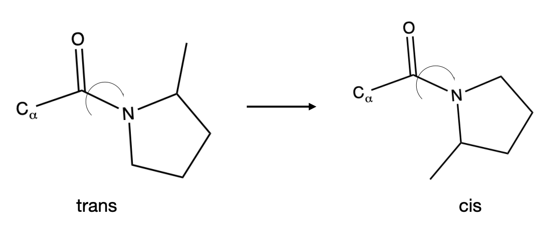
The number of reacting molecules in an elementary step determines the molecularity of the reaction. The molecularity of the reaction refers to a single elementary step in the mechanism that reflects what is actually happening in the reaction at a molecular level. An elementary step that involves only one reactant molecule are called unimolecular, and typically occurs with cis-trans isomerization, thermal decomposition, or ring-opening reactions. An example would be the decomposition of N₂O₄ (g) into NO₂ (g) according to the reaction:

\[\ce{N2O4 (g) → 2 NO2 (g)} \nonumber\]

For this example the rate would be

\[\text{rate}=\frac{1}{2}\frac{d[\text{NO}_2]}{dt}=k[\text{N}_2 \text{O}_4]\]

which is a first order reaction since the rate depends linearly on the concentration of the reactant N₂O₄ (g).

A second example is the conversion of trans proline to cis proline shown in Figure II.2.A

Figure II.2.A. The cis-trans isomerization of proline is an example of a unimolecular reaction.

An elementary step that involves two reactant molecules is called a bimolecular reaction. A simple example of a bimolecular reaction is reaction of H₂ (g) with I₂ (g) to form HI (g) according to the reaction:

\[\ce{H2 (g) + I2 (g) → 2 HI (g).} \nonumber\]

For this example, the rate is

\[\text{rate}=\frac{1}{2}\frac{d[\text{HI}]}{dt}=k[\text{H}_2][\text{I}_2]\]

An elementary step that involves the simultaneous encounter of three reactant molecules is called termolecular. Termolecular reactions are very rare because the probability of three reactant molecules colliding at the same time with the correct orientation and sufficient energy is very small. There are only a few known termolecular interactions, mostly involving nitric oxide. An example is the reaction of NO (g) with Cl₂ (g):

\[\ce{2 NO (g) + Cl2 (g) → 2 NOCl} \nonumber\]

For this example the reaction rate is

\[\text{rate}=\frac{1}{2}\frac{d[\text{NOCl}]}{dt}=k[\text{NO}]^2 [\text{Cl}_2]\]

which is overall a third-order reaction.

So far we have considered reaction mechanisms of individual, isolated reactions. In biochemistry, various elementary reaction steps are coupled or combined into complex reaction pathways. We will now look at a few of types of reaction pathways involving two or more reactions that can serve as building blocks for developing more complex reaction schemes.

Reversible Reaction

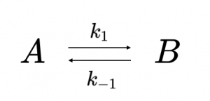
In a reversible reaction, the forward reaction (A → B) occurs with rate constant \(k_1\) while the reverse reaction (B → A) simultaneously occurs with rate constant \(k_{-1}\). The reversible reaction scheme is:

Reaction Scheme 1: Reversible Reaction

Examples of reactions of the type shown in Reaction Scheme 1 include protein folding and unfolding for a two-state model, a conformational change between an open and closed configuration of a protein, and a reversible isomerization reaction, such as the interconversion between dihydroxyacetone phosphate and glyceraldehyde-3-phosphate in glycolysis.

For a reaction scheme according to Reaction Scheme 1 the rate of change of the reactant is given by:

\[\frac{d[A]}{dt}=-k_1 [A] + k_{-1}[B]\label{EQ:reversible}\]

At equilibrium, the concentration of reactant and product become constant, and so there is no change in the concentration of A with time (\(d[A]/dt = 0\)), so at equilibrium:

\[k_1 [A] = k_{-1}[B]\label{EQ:equil1}\]

The ratio of [B]/[A] is the equilibrium constant \(K_{eq}\), leading to the expression:

\[\frac{[B]}{[A]} = K_{eq} = \frac{k_1}{k_{-1}}\label{EQ:equil2}\]

The relationship between the equilibrium constant and the forward and reverse reaction rates stems from the principle of microscopic reversibility that states that at equilibrium the rates of the forward and reverse process are equal for every elementary step of the reaction.

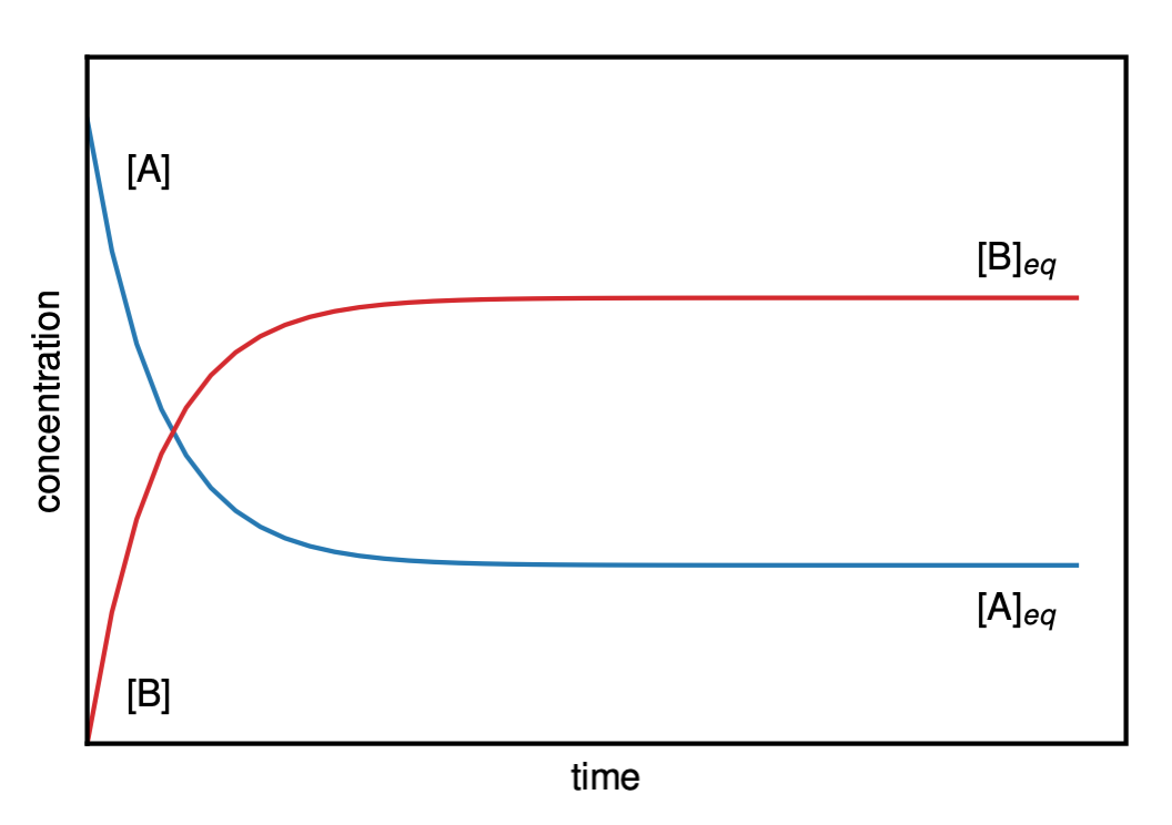
Figure II.2.B shows a plot of the concentration vs. time for a reaction according to Reaction Scheme 1. Before equilibrium, the concentrations of both A and B will change with time until the equilibrium state is reached, at which point the concentrations of A and B remain constant with a ratio given by Equation \ref{EQ:equil2}.

Figure II.2.B. Concentration of A and B vs. time for the reversible reaction according to Reaction Scheme 1. At equilibrium the rates of the forward and reverse reaction are equal, and the concentration of A and B are not changing. The ratio of [B]_eq and [A]_eq at equilibrium gives the equilibrium constant.

Another example is the bimolecular formation of a complex such as a ligand/protein complex:

Reaction Scheme 2: reversible bimolecular reaction

In this case the forward rate constant \(k_1\) is for a second order reaction with units of M\(^{-1}\) s\(^{-1}\) and the reverse rate constant \(k_{-1}\) is for a first order reaction with units of \(s^{-1}\). The rate constants for the complex formation is:

\[K_A = \frac{[AB]}{[A][B]}=\frac{k_1}{k_{-1}}\label{EQ:kA}\]

where \(K_A\) is the association constant (in units of M\(^{-1}\)), and for the dissociation:

\[K_D = \frac{[A][B]}{[AB]}=\frac{k_{-1}}{k_1}\label{EQ:kD}\]

where \(K_D\) is the dissociation constant (in units of M).

Parallel Reactions

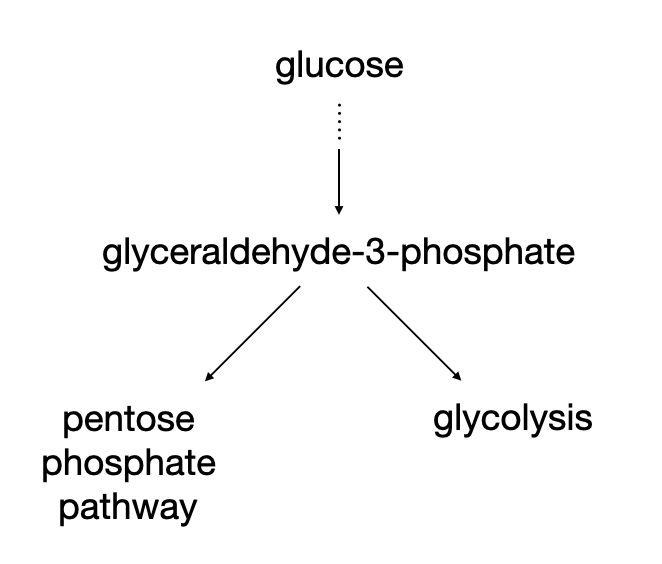
In metabolism, a metabolic precursor can be shunted into different metabolic pathways at a metabolic branching point. Consider for example that glyceraldehyde-3-phosphate (GAP) can be converted to 1,3-bisphosphoglycerate in the glycolysis pathway or can be used to convert sugars via the pentose phosphate pathway as shown in Figure II.2.C

Figure II.2.C. Example of a branching point in metabolism that leads to parallel reactions. Glucose is first converted to glyceraldehyde-3-phosphate which can enter the pentose phosphate pathway for the conversion of sugars or can be metabolized via glycolysis.

This kind of reaction scheme is a parallel reaction and there are numerous examples in metabolism. The overall reaction scheme is shown in Reaction Scheme 3:

Reaction Scheme 3: Parallel reaction

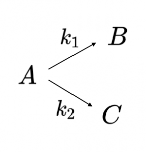
For the parallel reaction scheme of Reaction Scheme 3 the rate of consumption of A depends on both rate constants:

\[\begin{eqnarray}\frac{d[A]}{dt} &=& -k_1 [A] – k_2 [A] \nonumber \\[4pt] \frac{d[A]}{dt} &=& -(k_1 + k_2)[A] \label{EQ:parallel1}\end{eqnarray}\]

Equation \ref{EQ:parallel1} is a first order reaction that can be integrated to give:

\[[A] = [A]_0 e^{-(k_1 +k_2)t}\label{EQ:parallel2}\]

The rate of formation of the products B and C are given by:

\[\begin{eqnarray}\frac{d[B]}{dt} &=& k_1 [A] \nonumber \\[4pt] \frac{d[C]}{dt} &=& k_2 [A]\label{EQ:parallel3}\end{eqnarray}\]

Substitution of Equation \ref{EQ:parallel2} into Equation \ref{EQ:parallel3} gives after integration:

\[[B] = [A]_0 \frac{k_1}{k_1 + k_2}\left(1-e^{-(k_1 + k_2)t}\right)\label{EQ:parallel4}\]

and

\[[C] = [A]_0 \frac{k_2}{k_1 + k_2}\left(1-e^{-(k_1 + k_2)t}\right)\label{EQ:parallel5}\]

Figure II.2.D shows the concentrations as a function of time for the reactant A and the products B and C for a parallel reaction. Notice that [A] decrease to zero and gets used up, at which point the [B] and [C] remain constant, since there is no more reactant.

Figure II.2.D Concentration of A, B, and C vs. time for the parallel reaction according to Reaction Scheme 3. [A] decreases exponentially (first order kinetics) unit A is used up. When A is used up, [B] and [C] remain constant since there is no more reactant. The ratio of [B] or [C] formed can be determined from the ratio of rate constants k₁ and k₂.

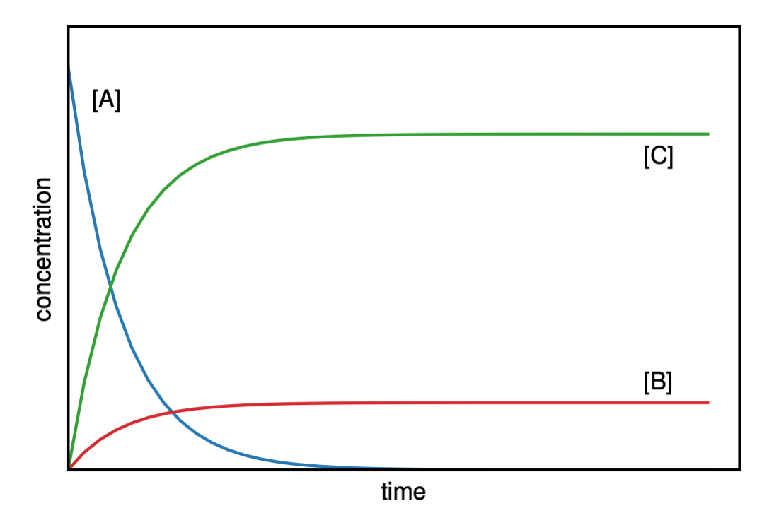
If we are interested in the final concentration of [B] and [C] after A is used up, (as shown in Figure II.2.D), we can take the limit of Equation \ref{EQ:parallel4} and Equation \ref{EQ:parallel5} as the time goes to infinity:

\[\begin{eqnarray}[B]_{\infty} &=& [A]_0 \frac{k_1}{k_1 + k_2} \nonumber \\[4pt] \left[ C \right]_{\infty} &=& [A]_0 \frac{k_2}{k_1 + k_2}\label{EQ:parallel6}\end{eqnarray}\]

From Equation \ref{EQ:parallel6} we see that the final concentration of [B] and [C] depends on the rate constants of the two parallel reactions (\(k_1\) and \(k_2\)). The ratio of rate constants is equal to the ratio of the final products:

\[\begin{eqnarray}\frac{[B]_{\infty}}{[C]_{\infty}}&=&\frac{[A]_0 \frac{k_1}{k_1 + k_2}}{[A]_0 \frac{k_2}{k_1 + k_2} } \nonumber \\[4pt] \frac{[B]_{\infty}}{[C]_{\infty}}&=& \frac{k_1}{k_2}\end{eqnarray}\]

See practice problem ???

Consecutive Reactions

Another common feature of metabolic pathways are consecutive reactions in which the product from the first step become the reactant for a second step, etc…. The metabolism of ethanol is an example. Ethanol is first oxidized to acetaldehyde by the enzyme alcohol dehydrogenase. In a second step, acetaldehyde is oxidized to acetic acid by acetaldehyde dehydrogenase:

The accumulation of acetaldehyde causes nausea and headaches.

For a two-step consecutive reaction of the form of Reaction Scheme 4:

Reaction Scheme 4: Consecutive reactions

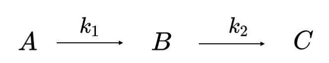
the rate law equations are:

\[\begin{eqnarray}\frac{d[A]}{dt}&=&-k_1 [A] \nonumber \\[4pt] \frac{d[B]}{dt}&=&k_1 [A] -k_2[B]\nonumber \\[4pt] \frac{d[C]}{dt}&=&k_2 [B]\label{EQ:consecutiverate1}\end{eqnarray}\]

Plots of the concentrations of A, B, and C as a function of time are shown in Figure II.2.E

Figure II.2.E. Concentration of A, B, and C vs. time for the consecutive reaction of Reaction Scheme 4. a) Case where k₁ < k_2. The conversion of B → C is much faster than the formation of B from A, therefore [B] does not build up. b) Case where k₁ > k₂. The reaction B → C is much slower than the formation of B from A, leading to accumulation of B.

From Figure II.2.E and from Equation \ref{EQ:consecutiverate1} we see that A decreases according the first-order rate law:

\[[A] = [A]_0 e^{-k_1 t}\label{EQ:firstorder1}\]

Equation \ref{EQ:firstorder1} can be substituted into the middle Equation \ref{EQ:consecutiverate1}, which can be integrated to give:

\[[B] = [A]_0 \frac{k_1}{k_2 – k_1}\left(e^{-k_1 t}-e^{-k_2 t}\right)\label{EQ:consecutivereactionB}\]

Finally, [C] can be determined from the conservation of mass requirement that \([C] = [A]_0 – [A] – [B]\) to obtain:

\[[C] = [A]_0 \left(1 + \frac{k_1 e^{-k_2 t}-k_2 e^{-k_1 t}}{k_2 – k_1} \right)\label{EQ:consecutivereactionC}\]

Figure II.2.D shows the time dependence of A, B, and C for Reaction Scheme 4. Notice that B is an intermediate and is only produced transiently. Eventually, the intermediate B will be used up and converted to C. The amount of accumulation of B depends on the relative rate constants \(k_1\) and \(k_2\). Figure II.2.E (a) shows the case where \(k_1 << k_2\). In this case, the conversion of B → C is much faster than the formation of B from A. In this case we see that the concentration of B does not appreciate because as soon as B is formed, it is converted into C. Figure II.2.E (b) shows the case where \(k_1 >> k_2\). In this case, the reaction B → C is much slower than the formation of B from A. In this case, B will initially accumulate until A is used up. Once A is used up, B begins to decrease as it is slowly converted into C.

Practice Problems

Problem 1. Initially a system has only species A at a concentration of 0.1 M. If a process proceeds from A to both B and C in parallel first-order reactions, and the forward rate to produce B is ten times larger than the rate to produce C, what are the final amounts of species B and C?

Problem 2. Consider the consecutive reaction in which ATP binds to an enzyme with a rate constant of \(k_1 = 0.3\) s\(^{-1}\) in the first step and then is hydrolyzed with a rate constant of \(k_2=1\times 10^{-3}\) s\(^{-1}\). a) Do you expect to be able to detect the intermediate ATP-bound enzyme complex? Why? b) Do How long is the lifetime of the intermediate ATP-bound enzyme complex?