1.5: The Boltzmann Distribution and the Statistical Definition of Entropy

In this chapter we introduce the statistical definition of entropy as formulated by Boltzmann. This allows us to consider entropy from the perspective of the probabilities of different configurations of the constituent interacting particles in an ensemble. This conception of entropy led to the development of modern statistical thermodynamics. For systems that can exchange thermal energy with the surroundings, the equilibrium probability distribution will be the Boltzmann distribution. Knowing this equilibrium probability distribution allows us to calculate various thermodynamics observables.

Learning Objectives

• Understand the statistical definition of entropy and be able to use the number of available microstates of the system to calculate the entropy.
• Understand how all thermodynamic properties ultimately can be traced back to the number of occupied microstates and their probability.
• Be able to use the Boltzmann distribution to calculate the ratio of occupied energy states at a given temperature and the probability of a particle being in any particular energy level.

Microstates and Boltzmann Entropy

In our discussion of thermodynamics, thus far we have neglected the molecular nature of reality: that molecular systems are composed of many interacting atoms. In this chapter we will explore how the large number of atoms in a macromolecular system gives rise to thermodynamic observables. We have seen that the thermodynamic state of the system can be designed by a set of state properties (P, V, n, T, U, H, S). The macroscopic state of the system is called a macrostate. In contrast, a microstate is a specific configuration of all the constituent atoms that make up the system.

As an illustrative example of a microstate is to consider the number of ways any given state may be constructed. Consider the question of how many unique ways there are to arrange four particles as shown in Figure I.5.A into two bins.

Figure I.5.A Consider the number of possible ways to arrange four particles into two bins. The are a total of 16 unique configurations as shown in Figure 1.5.B

It turns out that there are 16 different ways we could arrange four particles into two bins as shown in Figure I.5.B.

Figure I.5.B The total number of ways to arrange four particles into two bins. There are five possible macrostates defined by the number of particles in each bin ({4,0}, {3,1}, {2,2}, {1,3},{0,4}). Whereas the macrostate {4,0} can only be achieved in one way, the macrostate {2,2} can be achieved in six different ways.

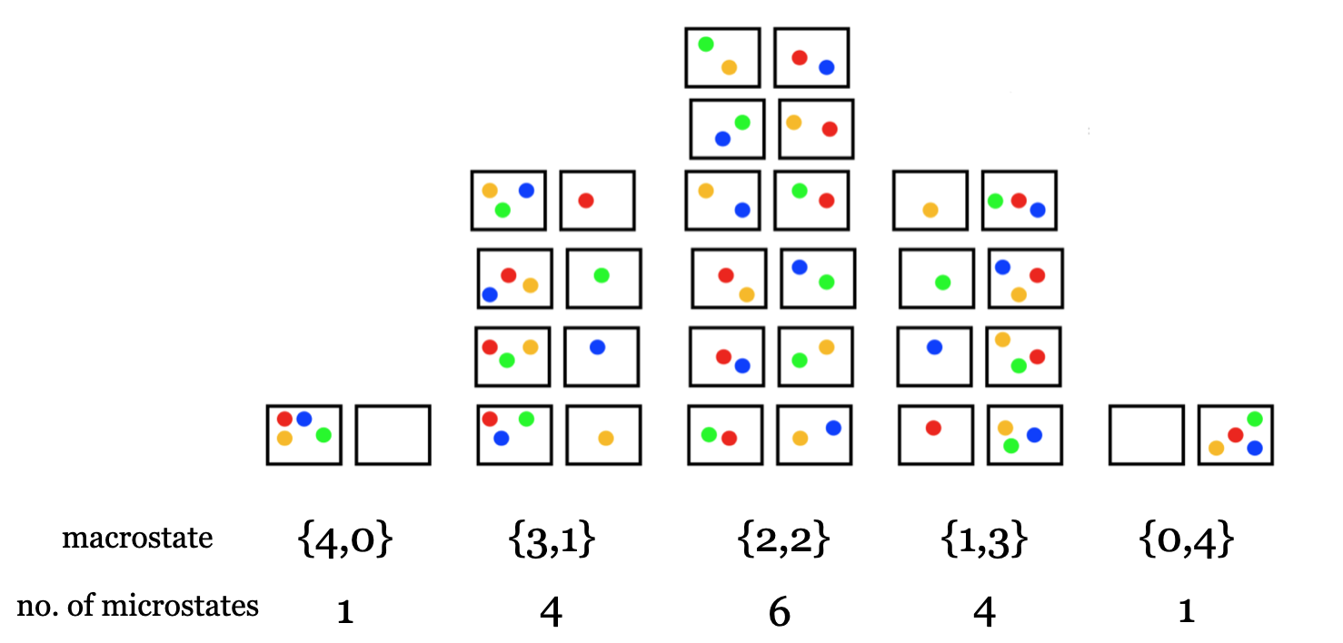
If we define each unique arrangement of the four particles as a microstate, then there are 16 possible microstates. The overall number of particles in each bin defines the macrostate, so from Figure I.5.B we see that there are four macrostates, and that the number of microstates making up the different macrostates is not equal. The macrostate that corresponds to a configuration with two particles in each bin ({2,2}) has the highest number of microstates (6), while the macrostates that correspond to configurations with all the particles in one of the bins ({4,0} and {0,4}) have the fewest number of microstates (1).

In general, we can calculate the number of microstates in a given distribution according to the formula:

\[W = \frac{N!}{n_1!n_2!,…}\label{EQ:statweight}\]

where W is the number of ways of distributing \(N\) total particles into bins, and \(n_1\), \(n_2\), … is the number of particles in each bin.

Example \(\PageIndex{1}\)

Example 1: Use Equation \ref{EQ:statweight} to calculate the number of ways to arrange four particles into two bins such that there are two particles in each bin ({2,2}).

Solution

We have four total particles, so \(N=4\). To calculate the number of ways to arrange four particles into a configuration with \(n_1=2\) and \(n_2=2\) we have:

\[\begin{eqnarray}W &=& \frac{4!}{2!2!} \nonumber \\[4pt] W &=& \frac{4\times 3\times 2 \times 1}{2\times 1 \times 2 \times 1} \nonumber \\[4pt] W &=& 6\end{eqnarray}\]

We calculate that there are six different microstates corresponding to the macrostate with two particles in each bin ({2,2}), which agrees with the drawing in Figure I.5.B.

See Practice Problems 1 and 2

The Boltzmann definition of entropy relates the entropy as the natural logarithm of the number of microstates, W:

\[S=k_B\ln W\label{EQ:BoltzmannS}\]

where \(\bf{k_B}\) is a constant of proportionality known as Boltzmann’s constant:

\[k_B = 1.380658 \times 10^{-23} \ \text{J K}^{-1}\]

Since W is unitless, the units on \(\bf{k_B}\) give entropy the correct thermodynamic units, and the value of Boltzmann’s constant ensures that the statistical definition of entropy from Equation \ref{EQ:BoltzmannS} is in agreement with the thermodynamic definition of entropy from Chapter I.4.

The Boltzmann Distribution

Equation \ref{EQ:BoltzmannS} allows us to compute the entropy \(\bf{S}\) for any given configuration of particles. Looking again at FigureI.5.B, we see that the configuration with two particles in each bin ({2,2}) has more accessible microstates (W=6) than a configuration with all four particles in one bin ({4,0} with W=1). Therefore, the macrostate with configuration {2,2} has a greater entropy than the macrostate with configuration {4,0}.

As a second example consider a system of four particles with two discrete energy levels as shown in Figure I.5.C.

Figure I.5.C: Two level system. Consider a system of four particles each with two accessible energy levels: a ground state energy with energy \(E_0\) and a single excited state with energy \(E_1\). If all particles are in the ground state, the total energy is \(E=4E_0\) as shown on the left. There is only one way to have all the particles in the ground state so W=1. If one of the particles is in the excited state, the total energy is \(E=3E_0 +E_1\) and W=4 since there are four possible ways to have a configuration with one particle in the excited state.

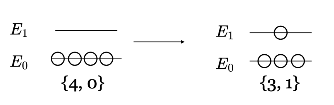
The particles can either be at the ground state energy \(E_0\) or the excited state energy \(E_1\). For example, the left side of Figure I.5.C shows the microstate with all four particles in the ground state. In this state, the total energy is \(E=4E_0\), and there is only one possible microstate (W=1). The configuration on the left corresponds to the macrostate with the lowest entropy. The right side of Figure I.5.C shows three particles in the ground state and one particle in the excited state. In the configuration on the right, the total energy is \(E=3E_0 + E_1\) and there are four possible microstates since any one our of the four particles could be in the excited state (W=4). The entropy of each of these configurations can be calculated from Equation \ref{EQ:BoltzmannS} using Equation I.5.\ref{EQ:statweight}.

We now ask ourselves, is there a dominant configuration of particles? The dominant configuration will be the configuration that maximizes \(\bf{W}\), or equivalently the configuration that maximizes the entropy \(\bf{S}\). Since W is a function of all the \(n_i\), the dominant configuration (that maximizes S) will be given by:

\[\left(\frac{\partial \ln W}{\partial n_i}\right)=0\label{EQ:maxS}\]

where \(\bf{n_i}\) is the number of particles in energy level \(i\).

In solving for the maximum entropy condition of Equation \ref{EQ:maxS}, we must also enforce the constraint that the total energy of the system is:

\[E_{total} = \sum_i n_i E_i\label{EQ:constantE}\]

and that the total number of particles \(\bf{N}\) is:

\[N = \sum_i n_i\label{EQ:constantN}\]

Maximizing a function subject to constraints can be done using a mathematical technique called Lagrange’s method of undetermined multipliers. The result is that at a given temperature \(\bf{T}\), the fraction of particles with energy \(E_i\) is given by:

\[\frac{n_i}{N}=\frac{e^{-E_i/k_BT}}{q}.\label{EQ:Boltzmann}\]

Equation \ref{EQ:Boltzmann} is known as the Boltzmann distribution and gives the probability of a particle occupying a given energy level \(\bf{E_i}\) at temperature \(\bf{T}\). The term in the denominator \(\bf{q}\) is called the partition function and is given by:

\[q=\sum_i e^{-E_i/k_BT}= e^{-E_0/k_BT}+e^{-E_1/k_BT}+…\]

The ratio of the number of particles (populations) between any two energy levels \(\bf{n_1}\) and \(\bf{n_2}\) is given by:

\[\frac{n_2}{n_1}=e^{-\Delta E/k_BT}\label{EQ:Boltzmann2}\]

where \(\bf{\Delta E}\) is the difference in energy between the two energy levels \(\Delta E=E_2 – E_1\)

Key Result: The Boltzmann distribution gives the distribution of particles that corresponds to the most probable populations and is given by the formula: \[ \frac{n_i}{N}=\frac{e^{-E_i/k_BT}}{\sum_i e^{-E_i/k_BT}}. \nonumber \]

The ratio of the number of particles between any two energy levels is

\[ \frac{n_2}{n_1}=e^{-\Delta E/k_BT}. \nonumber \]

See Practice Problem 3

Degenerate Energy Levels

Equation \ref{EQ:Boltzmann} and Equation \ref{EQ:Boltzmann2} were derived without considering the case of degeneracy. In practice, there may be two or more distinct states with the same energy. Two distinct states with the same energy are called degenerate energy levels. We specify the degeneracy of a particular energy level \(i\) with the symbol \(\bf{g_i}.\) Figure I.5.D shows a situation where the ground state is not degenerate (\(\bf{g_0=1}\)), and the excited state has a degeneracy of \(\bf{g_1=2}\) because there are two possible states with the same energy \(E_1.\)

Figure I.5.D. Degenerate energy levels: In this example there is only one ground state level with energy \(E_0\), but there are two possible excited state energy levels with the same energy \(E_1\). A particle in the ground state can be excited into either of the two excited states. Because these two states have the same energy they are called degenerate energy levels. In this example, the excited state \(E_1\) has a degeneracy \(g_1=2\) while the ground state has a degeneracy \(g_0=1\).

For the case where there are degenerate energy levels, we generalize the probabilities given by Equation \ref{EQ:Boltzmann} and Equation I.5.\ref{EQ:Boltzmann2}. The general Boltzmann distribution will be:

\[\frac{n_i}{N}=\frac{g_i e^{-E_i/k_BT}}{q}.\label{EQ:Boltzmann_degenerate}\]

with \(g_i\) the degeneracy of state \(i\) and the partition function:

\[q=\sum_i g_i e^{-E_i/k_BT}= g_0 e^{-E_0/k_BT}+g_1 e^{-E_1/k_BT}+…\label{EQ:partition_degenerate}\]

The ratio of the number of particles (populations) between any two energy levels \(\bf{n_1}\) and \(\bf{n_2}\) is given by:

\[\frac{n_2}{n_1} =\frac{g_2}{g_1}e^{-\Delta E/k_BT} \]

Examples

Example \(\PageIndex{2}\)

Calculate the number of microstates for 8 particles to be arranged into 4 bins such that the configuration of particles is {6,0,0,2}

Solution

The number of microstates is given by Equation \ref{EQ:statweight}:

\(W = \frac{N!}{n_1!n_2!,…}\)

\(W = \frac{8!}{6!0!0!2!} \)

\( W = 28 \)

Example \(\PageIndex{2}\)

a) Write an expression for the partition function for the two-level system shown in Figure I.5.D with energy in the ground state \(E_0 \) and degeneracy \(g_0 = 1 \) and energy in the excited state \(E_1 \) and degeneracy \(g_1 = 2 \). b) Let the energy of the ground state be \(E_0 =0\) and the energy in the excited state be \(E_1 = 2.41 \) kJ mol\(^{-1}\). Evaluate the value of the partition function at T=298 K. c) What is the probability to find the system in the ground state at T=298 K?

Solution

a) Using Equation \ref{EQ:partition_degenerate}, for a two-level system we have:

\( q = g_0 e^{-E_0/k_BT} + g_1 e^{-E_1/k_BT} \)

and substituting the values of the degeneracy gives:

\(q = e^{-E_0/k_BT} + 2 e^{-E_1/k_BT} \)

b) When energies are given in molar units (kJ mol\(^{-1}\)), it is useful to use the gas constant \(R = 8.314\) J mol\(^{-1}\) K\(^{-1} = N_A k_B \). The the partition function becomes:

\(q = 1 + 2 e^{-2410/(8.314 \cdot 298)} \)

\(q = 1.756 \)

c) The probability for the system to be in the ground state is given by Equation \ref{EQ:Boltzmann_degenerate}:

\( p_0 = \frac{g_0 e^{-E_0/k_BT}}{q} \)

\( p_0 = \frac{1}{q} \)

Inserting the value of q from part b):

\(p_0 = 0.569 \)

Practice Problems

Problem 1. Calculate the total number of ways to arrange 16 particles into four bins such that there are four particles in each bin ({4,4,4,4}). What can you say about the entropy of this macrostate as compared to any other macrostate? Explain your answer.

Problem 2. Suppose we have 8 particles that are arranged into 4 bins. Calculate the number of microstates (W) for each of the following distributions of particles: a) {5,1,1,1}, b) {4,2,2,0}, c) {2,6,0,0}

Problem 3. Suppose a protein can exist in two conformations that have an energy difference of 2.0 kJ/mol. What is the estimated ratio of the two conformations at 300 K?

Problem 4.